Dog vs Cat Classification with CNN

Use of Dropout and Batch Normalization in 2D CNN on Dog Cat Image Classification in TensorFlow 2.0

We are going to predict cat or dog by the help of Convolutional neural network. The dataset is sourced from the Kaggle Cat and Dog dataset. In this dataset there is two class cats and dogs and we have to predict whether the cat or dog by the help of CNN algorithm.

Download Data from GitHub and Model Building

We are going to use tensorflow 2.3 (which is the latest version) to build the model. You can install TensorFlow by running this command.

!pip install tensorflow-gpu==2.3.0-rc0

Importing necessary library that will use in model building.

import tensorflow as tf
from tensorflow import keras
from tensorflow.keras import Sequential
from tensorflow.keras.layers import Flatten, Dense, Conv2D, MaxPool2D, ZeroPadding2D, Dropout, BatchNormalization
from tensorflow.keras.preprocessing.image import ImageDataGenerator

from tensorflow.keras.optimizers import SGD

print(tf.__version__)

2.3.0

pandas for loading and manipulating the data.

pyplot from matplotlib is used to visualize the results.

import numpy as np
import matplotlib.pyplot as plt

git clone is a Git command-line utility that is used to target an existing repository and create a clone, or copy of the target repository.

!git clone https://github.com/laxmimerit/dog-cat-full-dataset.git

Cloning into 'dog-cat-full-dataset'...
remote: Enumerating objects: 25027, done.
remote: Total 25027 (delta 0), reused 0 (delta 0), pack-reused 25027
Receiving objects: 100% (25027/25027), 541.62 MiB | 37.27 MiB/s, done.
Resolving deltas: 100% (5/5), done.
Checking out files: 100% (25001/25001), done.

test_data_dir = '/content/dog-cat-full-dataset/data/test'
train_data_dir = '/content/dog-cat-full-dataset/data/train'

Size of these images are quite large due to limited resources we are going to resize the image in the 32 x 32.

img_width = 32
img_height = 32
batch_size = 20

ImageDataGenerator generates batches of image data with real-time data augmentation. We are giving argument to rescale the image pixel from 255 to 1 then learning very fast.

datagen = ImageDataGenerator(rescale=1./255)

We are going to read the images to numerical array from the directory and in the argument we are passing the path of train_data_dir then after passing target_size that means which size it should read the images then after classes have two class i.e. dogs and cats and in class_mode we are giving binary because it has binary problem and at last batch_size we are passing 20 value.

train_generator = datagen.flow_from_directory(directory=train_data_dir,
                                              target_size = (img_width, img_height),
                                              classes = ['dogs', 'cats'],
                                              class_mode = 'binary',
                                              batch_size=batch_size)

Found 20000 images belonging to 2 classes.

It will give the class i.e. it has two class 0 and 1(Dogs and Cats).

train_generator.classes

array([0, 0, 0, ..., 1, 1, 1], dtype=int32)

Now, we will using for validation purpose. datagen.flow_directory function we are passing argument test_data_dir directory then after passing target_size that means which size it should read the images then after classes have two class i.e. dogs and cats and in class_mode we are giving binary because it has binary problem and at last batch_size we are passing 20 value.

validation_generator = datagen.flow_from_directory(directory=test_data_dir,
                                                   target_size = (32, 32),
                                                   classes = ['dogs', 'cats'],
                                                   class_mode = 'binary',
                                                   batch_size = batch_size)

Found 5000 images belonging to 2 classes.

Let's go to see the length of data_generator.

data_generator = train_generator * batch_size

len(train_generator)*batch_size

20000

Now, Let's go ahead and build our first CNN model

Build CNN Base Model

A Sequential() function is the easiest way to build a model in Keras. It allows you to build a model layer by layer. Each layer has weights that correspond to the layer the follows it. We use the add() function to add layers to our model.

A 2D convolution layer means that the input of the convolution operation is three-dimensional, for example, a color image that has a value for each pixel across three layers: red, blue and green. However, it is called a 2D convolution because the movement of the filter across the image happens in two dimensions.

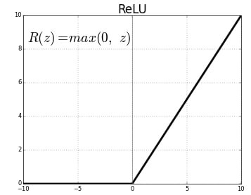
The Rectified Linear Unit(ReLu) is the most commonly used activation function in deep learning models. The function returns 0 if it receives any negative input, but for any positive value x it returns that value back. So it can be written as f(x)=max(0,x)

To stop problem of shrinkage of data we use concept called Padding.

It has two types:

• valid
• same

Max pooling is a sample-based discretization process. The objective is to down-sample an input representation (image, hidden-layer output matrix, etc.), reducing its dimensionality and allowing for assumptions to be made about features contained in the sub-regions binned. This is done to in part to help over-fitting by providing an abstracted form of the representation. As well, it reduces the computational cost by reducing the number of parameters to learn and provides basic translation invariance to the internal representation.

Flattening is converting the data into a 1-dimensional array for inputting it to the next layer. We flatten the output of the convolutional layers to create a single long feature vector.

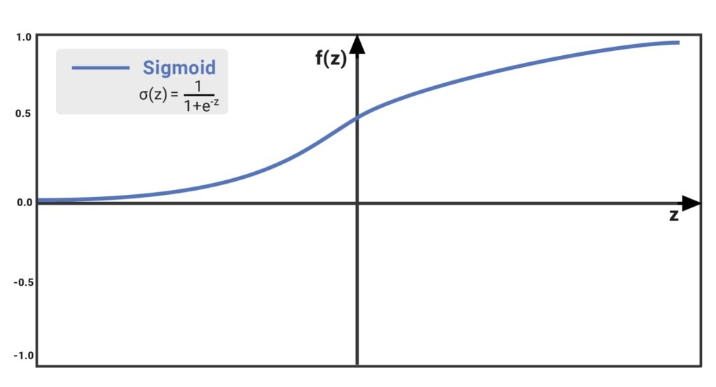
The Sigmoid function takes a value as input and outputs another value between 0 and 1. It is non-linear and easy to work with when constructing a neural network model. The good part about this function is that continuously differentiable over different values of z and has a fixed output range.

model = Sequential()
model.add(Conv2D(filters=64, kernel_size=(3,3), activation='relu', padding='same', kernel_initializer='he_uniform', input_shape = (img_width, img_height, 3)))
model.add(MaxPool2D(2,2))

model.add(Flatten())
model.add(Dense(128, activation='relu', kernel_initializer='he_uniform'))
model.add(Dense(1, activation='sigmoid'))

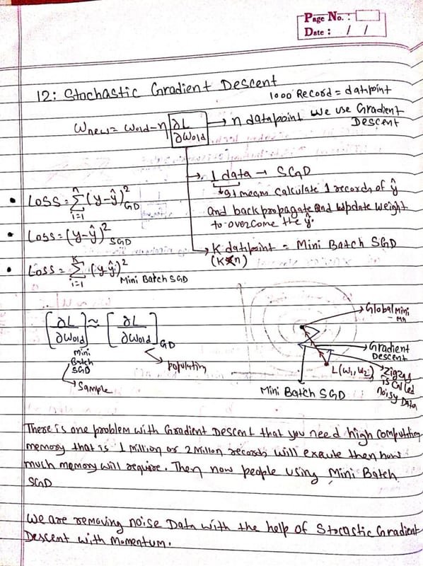
The diagram below shows the key differences between Gradient Descent, Stochastic Gradient Descent, and Mini-Batch SGD, which is the optimizer variant used here:

Compile defines the loss function, the optimizer and the metrics. That's all. It has nothing to do with the weights and you can compile a model as many times as you want without causing any problem to pretrained weights.

opt = SGD(learning_rate=0.01, momentum=0.9)
model.compile(optimizer=opt, loss='binary_crossentropy', metrics=['accuracy'])

The model.fit_generator() function accepts the batch of data, performs backpropagation, and updates the weights in our model. This process is repeated until we have reached the desired number of epochs.

history = model.fit_generator(generator=train_generator, steps_per_epoch=len(train_generator), epochs = 5, validation_data=validation_generator, validation_steps=len(validation_generator), verbose = 1)

WARNING:tensorflow:From :1: Model.fit_generator (from tensorflow.python.keras.engine.training) is deprecated and will be removed in a future version.
Instructions for updating:
Please use Model.fit, which supports generators.
Epoch 1/5
1000/1000 [==============================] - 100s 100ms/step - loss: 0.6971 - accuracy: 0.5077 - val_loss: 0.6926 - val_accuracy: 0.5000
Epoch 2/5
1000/1000 [==============================] - 99s 99ms/step - loss: 0.6892 - accuracy: 0.5205 - val_loss: 0.6898 - val_accuracy: 0.5320
Epoch 3/5
1000/1000 [==============================] - 100s 100ms/step - loss: 0.6760 - accuracy: 0.5673 - val_loss: 0.6754 - val_accuracy: 0.5724
Epoch 4/5
1000/1000 [==============================] - 99s 99ms/step - loss: 0.6068 - accuracy: 0.6747 - val_loss: 0.5471 - val_accuracy: 0.7260
Epoch 5/5
1000/1000 [==============================] - 99s 99ms/step - loss: 0.5346 - accuracy: 0.7325 - val_loss: 0.5180 - val_accuracy: 0.7474

history.history

{'accuracy': [0.5077000260353088, 0.5205000042915344, 0.567300021648407, 0.6747000217437744, 0.732450008392334], 'loss': [0.6971414089202881, 0.6891948580741882, 0.6759502291679382, 0.6068235635757446, 0.5346073508262634], 'val_accuracy': [0.5, 0.5320000052452087, 0.5723999738693237, 0.7260000109672546, 0.7473999857902527], 'val_loss': [0.692634642124176, 0.6898210644721985, 0.6753650903701782, 0.5471111536026001, 0.5179951190948486]}

def plot_learningCurve(history):
  # Plot training & validation accuracy values
  epoch_range = range(1, 6)
  plt.plot(epoch_range, history.history['accuracy'])
  plt.plot(epoch_range, history.history['val_accuracy'])
  plt.title('Model accuracy')
  plt.ylabel('Accuracy')
  plt.xlabel('Epoch')
  plt.legend(['Train', 'Val'], loc='upper left')
  plt.show()

  # Plot training & validation loss values
  plt.plot(epoch_range, history.history['loss'])
  plt.plot(epoch_range, history.history['val_loss'])
  plt.title('Model loss')
  plt.ylabel('Loss')
  plt.xlabel('Epoch')
  plt.legend(['Train', 'Val'], loc='upper left')
  plt.show()

In the Model loss fig. validation loss is always less than training loss that means our model is underfitting. And in Model Accuracy fig you are seeing accuracy of validation set is greater than training set then our model is not overfitting at all and we can increase the no. of epochs.

plot_learningCurve(history)

Implement First 3 Blocks of VGG16 Model

We are going to implement 3 blocks of VGG16 Model.

• In the first block, it has to take 64 filters.
• In the second block, we are taking 128 filters.
• And at the last third block, we are going to use 256 filters.

model = Sequential()
model.add(Conv2D(filters=64, kernel_size=(3,3), activation='relu', padding='same', kernel_initializer='he_uniform', input_shape = (img_width, img_height, 3)))
model.add(MaxPool2D(2,2))

model = Sequential()
model.add(Conv2D(filters=128, kernel_size=(3,3), activation='relu', padding='same', kernel_initializer='he_uniform'))
model.add(MaxPool2D(2,2))

model = Sequential()
model.add(Conv2D(filters=256, kernel_size=(3,3), activation='relu', padding='same', kernel_initializer='he_uniform'))
model.add(MaxPool2D(2,2))

model.add(Flatten())
model.add(Dense(128, activation='relu', kernel_initializer='he_uniform'))

model.add(Dense(1, activation='sigmoid'))

opt = SGD(learning_rate=0.01, momentum=0.9)
model.compile(optimizer=opt, loss='binary_crossentropy', metrics=['accuracy'])

history = model.fit_generator(generator=train_generator, steps_per_epoch=len(train_generator), epochs = 5, validation_data=validation_generator, validation_steps=len(validation_generator), verbose = 1)

Epoch 1/5
1000/1000 [==============================] - 174s 174ms/step - loss: 0.7074 - accuracy: 0.4951 - val_loss: 0.6932 - val_accuracy: 0.5000
Epoch 2/5
1000/1000 [==============================] - 177s 177ms/step - loss: 0.6935 - accuracy: 0.4978 - val_loss: 0.6932 - val_accuracy: 0.5000
Epoch 3/5
1000/1000 [==============================] - 179s 179ms/step - loss: 0.6934 - accuracy: 0.5002 - val_loss: 0.6931 - val_accuracy: 0.4998
Epoch 4/5
1000/1000 [==============================] - 175s 175ms/step - loss: 0.6935 - accuracy: 0.4945 - val_loss: 0.6950 - val_accuracy: 0.5000
Epoch 5/5
1000/1000 [==============================] - 172s 172ms/step - loss: 0.6936 - accuracy: 0.4969 - val_loss: 0.6931 - val_accuracy: 0.5002

With the help of this approach we got very very bad accuracy. Our val_accuracy is 50% and training accuracy also got approx 50%. Since this is a binary classification and 50% accuracy means our model is guessing a random basis. This happened because we implemented a very complex model on the small dataset.

To increase the accuracy we are going to add Batch Normalization and Dropout to achieve better accuracy.

Batch Normalization and Dropout

model = Sequential()
model.add(Conv2D(filters=64, kernel_size=(3,3), activation='relu', padding='same', kernel_initializer='he_uniform', input_shape = (img_width, img_height, 3)))
model.add(BatchNormalization())
model.add(MaxPool2D(2,2))
model.add(Dropout(0.2))

model = Sequential()
model.add(Conv2D(filters=128, kernel_size=(3,3), activation='relu', padding='same', kernel_initializer='he_uniform'))
model.add(BatchNormalization())
model.add(MaxPool2D(2,2))
model.add(Dropout(0.3))

model = Sequential()
model.add(Conv2D(filters=256, kernel_size=(3,3), activation='relu', padding='same', kernel_initializer='he_uniform'))
model.add(BatchNormalization())
model.add(MaxPool2D(2,2))
model.add(Dropout(0.5))

model.add(Flatten())
model.add(Dense(128, activation='relu', kernel_initializer='he_uniform'))
model.add(BatchNormalization())
model.add(Dropout(0.5))

model.add(Dense(1, activation='sigmoid'))

opt = SGD(learning_rate=0.01, momentum=0.9)
model.compile(optimizer=opt, loss='binary_crossentropy', metrics=['accuracy'])

history = model.fit_generator(generator=train_generator, steps_per_epoch=len(train_generator), epochs = 10, validation_data=validation_generator, validation_steps=len(validation_generator), verbose = 1)

Epoch 1/10
1000/1000 [==============================] - 239s 239ms/step - loss: 0.6800 - accuracy: 0.6283 - val_loss: 0.6531 - val_accuracy: 0.6644
...
Epoch 5/10
1000/1000 [==============================] - 240s 240ms/step - loss: 0.5136 - accuracy: 0.7496 - val_loss: 0.5080 - val_accuracy: 0.7592
Epoch 6/10
1000/1000 [==============================] - 239s 239ms/step - loss: 0.5006 - accuracy: 0.7584 - val_loss: 0.5198 - val_accuracy: 0.7514
Epoch 7/10
1000/1000 [==============================] - 242s 242ms/step - loss: 0.4929 - accuracy: 0.7609 - val_loss: 0.5420 - val_accuracy: 0.7270
Epoch 8/10
1000/1000 [==============================] - 240s 240ms/step - loss: 0.4957 - accuracy: 0.7623 - val_loss: 0.5901 - val_accuracy: 0.7068
Epoch 9/10
1000/1000 [==============================] - 243s 243ms/step - loss: 0.4846 - accuracy: 0.7678 - val_loss: 0.5548 - val_accuracy: 0.7288
Epoch 10/10
1000/1000 [==============================] - 240s 240ms/step - loss: 0.4648 - accuracy: 0.7781 - val_loss: 0.5182 - val_accuracy: 0.7406

We add Batch Normalisation and Dropout then i got little bit high accuracy from previous one then its good. And we also increases the epochs from 5 to 10 to achieve high accuracy.

def plot_learningCurve(history, epoch):
  # Plot training & validation accuracy values
  epoch_range = range(1, epoch+1)
  plt.plot(epoch_range, history.history['accuracy'])
  plt.plot(epoch_range, history.history['val_accuracy'])
  plt.title('Model accuracy')
  plt.ylabel('Accuracy')
  plt.xlabel('Epoch')
  plt.legend(['Train', 'Val'], loc='upper left')
  plt.show()

  # Plot training & validation loss values
  plt.plot(epoch_range, history.history['loss'])
  plt.plot(epoch_range, history.history['val_loss'])
  plt.title('Model loss')
  plt.ylabel('Loss')
  plt.xlabel('Epoch')
  plt.legend(['Train', 'Val'], loc='upper left')
  plt.show()

plot_learningCurve(history, 10)

In the Model accuracy fig. The accuracy of training data has kept increasing but the accuracy of validation data stops after 5 or 6 epochs.

In the Model loss fig. After 5 epochs validation loss starts increasing than training loss.

So moreover this learning curve we can identify that our model has started overfitting.

Note: In this Blog you definitely learn that Dropout and Batch Normalisation has great impact on Deep Neural Network.

Conclusion

In this tutorial you trained a 2D CNN to classify dog and cat images, progressing through three model variants: a basic Conv2D baseline (~73% validation accuracy), a 3-block VGG16-style model (50% — too complex for the dataset), and a 3-block model with BatchNormalization and Dropout (~74% at epoch 5 before overfitting). The learning curves clearly showed overfitting setting in after epoch 5.

Key takeaways:

• Matching model depth to dataset size is critical — a deep VGG-style architecture collapsed to random guessing on 20,000 images without regularization.
• BatchNormalization and Dropout together recovered meaningful learning but could not prevent overfitting past epoch 5; stronger augmentation is needed for further improvement.
• ImageDataGenerator with rescale=1./255 is the minimum preprocessing pipeline for image classification; adding flipping, rotation, and zoom augmentation would noticeably reduce overfitting.

Next steps:

• Use transfer learning with VGG-16 for Image Classification to achieve substantially higher accuracy without training from scratch.
• Apply multi-class image classification with CNN on CIFAR-10 to extend the same CNN concepts to 10 categories.
• Add horizontal flipping and random zoom to the ImageDataGenerator to reduce the overfitting gap seen after epoch 5.