Prediction of number of passengers for an airline using LSTM
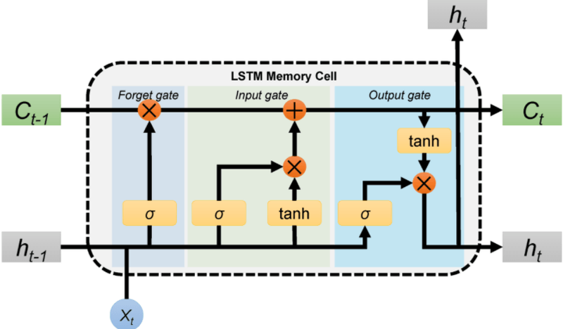
In this blog, we will build an LSTM regression model in TensorFlow to predict monthly airline passenger counts from the classic 1949-1960 dataset. Long Short-Term Memory (LSTM) networks keep context across long sequences through input, forget, and output gates, which makes them strong for time-series forecasting.
Dataset
This dataset provides monthly totals of a US airline passengers from 1949 to 1960. The dataset has 2 columns month and passengers. month contains the month of the year and passengers contains total number of passengers travelled on that particular month.
We can download the dataset from here.
Install tensorflow with the command below. If the machine has a GPU, use the second command.
!pip install tensorflow
!pip install tensorflow-gpu
import numpy as np
import matplotlib.pyplot as plt
import pandas as pd
from tensorflow.keras.models import Sequential
from tensorflow.keras.layers import Dense, LSTM
from sklearn.preprocessing import MinMaxScaler
Read the dataset using read.csv(). Only the passengers column is retained and reshaped by converting it into a numpy array.
dataset = pd.read_csv('AirPassengers.csv')
dataset = dataset['#Passengers']
dataset = np.array(dataset).reshape(-1,1)
dataset[:10]array([[112],
[118],
[132],
[129],
[121],
[135],
[148],
[148],
[136],
[119]], dtype=int64)Plotting the dataset shows that passenger numbers increased linearly over the period.
plt.plot(dataset)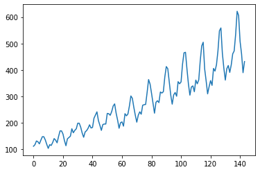
Neural networks work better if inputs are between 0 and 1. Scaling down the inputs with MinMaxScaler() produces a minimum value of 0 and maximum value of 1.
scaler = MinMaxScaler()
dataset = scaler.fit_transform(dataset)
dataset.min(),dataset.max()(0.0, 1.0)The first 100 months are used as training data and the last 44 months as testing data.
train_size = 100
test_size = 44
train = dataset[0:train_size, :]
train.shape(100, 1)test = dataset[train_size:144, :]
test.shape(44, 1)Create training and testing dataset
The model predicts the (i)th value based on the (i-1)th value, looking back by 1 to predict the next value. The function get_data() creates dataX and dataY for both the training and testing data.
def get_data(dataset, look_back):
    dataX, dataY = [], []
    for i in range(len(dataset)-look_back-1):
        a = dataset[i:(i+look_back), 0]
        dataX.append(a)
        dataY.append(dataset[i+look_back, 0])
    return np.array(dataX), np.array(dataY)

look_back = 1
X_train, y_train = get_data(train, look_back)
X_train[:10]array([[0.01544402],
[0.02702703],
[0.05405405],
[0.04826255],
[0.03281853],
[0.05984556],
[0.08494208],
[0.08494208],
[0.06177606],
[0.02895753]])y_train[:10]array([0.02702703, 0.05405405, 0.04826255, 0.03281853, 0.05984556,
0.08494208, 0.08494208, 0.06177606, 0.02895753, 0. ])The get_data() function is called again to create the testing data.
X_test, y_test = get_data(test, look_back)Reshape the data into 3 dimensions using reshape().
X_train = X_train.reshape(X_train.shape[0], X_train.shape[1], 1)
X_test = X_test.reshape(X_test.shape[0], X_test.shape[1], 1)X_train.shape(98, 1, 1)Build the model
The sequential model has 2 layers.
LSTM layer:
This is the main layer of the model and has 5 units. It learns long-term dependencies between time steps in time series and sequence data. input_shape contains the shape of input which must be passed as a parameter to the first layer of the neural network.
Dense layer:
Dense layer is the regular deeply connected neural network layer. It is most common and frequently used layer. The number of units is 1 because the output is a single value.
model = Sequential()
model.add(LSTM(5, input_shape = (1, look_back)))
model.add(Dense(1))
model.compile(loss = 'mean_squared_error', optimizer = 'adam')
The summary is available via model.summary().
model.summary()Model: "sequential"
_________________________________________________________________
Layer (type) Output Shape Param #
=================================================================
lstm (LSTM) (None, 5) 140
_________________________________________________________________
dense (Dense) (None, 1) 6
=================================================================
Total params: 146
Trainable params: 146
Non-trainable params: 0
_________________________________________________________________After compiling the model, train it using model.fit() on the training dataset with 50 epochs. An epoch is an iteration over the entire x and y data provided. batch_size is the number of samples per gradient update, meaning the weights update after every training example.
model.fit(X_train, y_train, epochs=50, batch_size=1)

Epoch 45/50
98/98 [==============================] - 0s 2ms/sample - loss: 0.0022
Epoch 46/50
98/98 [==============================] - 0s 2ms/sample - loss: 0.0021
Epoch 47/50
98/98 [==============================] - 0s 2ms/sample - loss: 0.0021
Epoch 48/50
98/98 [==============================] - 0s 2ms/sample - loss: 0.0021
Epoch 49/50
98/98 [==============================] - 0s 2ms/sample - loss: 0.0022
Epoch 50/50
98/98 [==============================] - 0s 2ms/sample - loss: 0.0021
Testing the model uses X_test.
y_pred = model.predict(X_test)This is the scaler value used earlier.
scaler.scale_array([0.0019305])The values were scaled before passing them to the neural network. To recover the original values, use scaler.inverse_transform().
y_pred = scaler.inverse_transform(y_pred)
y_test = np.array(y_test)
y_test = y_test.reshape(-1, 1)
y_test = scaler.inverse_transform(y_test)
The chart below compares real values against predicted values.
# plot baseline and predictions
plt.figure(figsize=(14,5))
plt.plot(y_test, label = 'Real number of passengers')
plt.plot(y_pred, label = 'Predicted number of passengers')
plt.ylabel('# passengers')
plt.legend()
plt.show()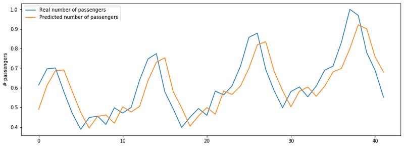
The actual results and the predicted results follow the same trend, with the model predicting passenger numbers at a good accuracy.
Conclusion
In this blog, we built a single-layer LSTM regressor in TensorFlow to predict monthly airline passenger counts from the classic 1949-1960 dataset. We used a look-back window of 1 and MinMaxScaler normalization. The model learned the upward trend and the seasonal pattern, and its predictions closely tracked the real values on the 44-month test set.
Key takeaways:
MinMaxScaleris essential before feeding time-series data into an LSTM. Unnormalized values destabilize gradient updates.- A look-back window of 1 captures only the previous step; increasing it lets the model see longer seasonal cycles at the cost of more training data.
- Always apply
inverse_transformbefore evaluating predictions so RMSE is in the original passenger-count scale, not the 0-1 normalized range.
Next steps:
- Extend to multi-step forecasting in Multi-Step Time Series Prediction with LSTM to predict an entire week of values at once.
- Apply the same LSTM approach to financial data in Google Stock Price Prediction using RNN-LSTM.
- Try stacking two LSTM layers with Dropout between them to capture higher-level temporal patterns in the series.


