Getting Started with TensorFlow 2.0 and Keras

Classification using *Fashion MNIST * dataset

TensorFlow 2.0 is Google's open-source deep learning framework, now powered by Keras as its high-level API. It brings eager execution, cleaner APIs, and faster iteration compared to TF 1.x.

Install with pip install tensorflow (or pip install tensorflow-gpu for GPU).

Fashion MNIST dataset

We are going to use the Fasion Mnist dataset. It consists of a training set of 60,000 examples and a test set of 10,000 examples. All the 70,000 images show individual articles of clothing at low resolution (28 by 28 pixels). The grayscale images are from 10 categories(T-shirt/top, Trouser, Pullover, Dress, Coat, Sandal, Shirt, Sneaker, Bag, Ankle boot) as seen here:

You can download the actual dataset from here.

In this notebook we are goint to use the fashion_mnist dataset which is available in keras.

import tensorflow as tf
from tensorflow import keras

print(tf.__version__)

2.1.0

import numpy as np
import pandas as pd
import matplotlib.pyplot as plt

Here we are loading the fashion_mnist dataset from keras.

mnist = keras.datasets.fashion_mnist

The dataset is downloaded in TFModuleWrapper.

type(mnist)

module

Now we load the data into real variables using load_data(). It return 2 tuples. The first tupes has the training data and the second tuple has the test data.

(X_train, y_train), (X_test, y_test) = mnist.load_data()

By using shape we can see that it has 60,000 images for training and each image is of size 28x28 in X_train and a corresponding label for each image in y_train.

X_train.shape, y_train.shape

((60000, 28, 28), (60000,))

np.max() gives the maximum value. Hence the maximum value in X_train is 255. We can even see the minimum value using np.min(X_train). The minimum value will be 0.

np.max(X_train)

255

np.mean() gives the mean value. The mean value in X_train is 72.94

np.mean(X_train)

72.94035223214286

As we know the images are divided into 10 categories. The 10 categories are encoded using a numerical value as show below.

y_train

array([9, 0, 0, ..., 3, 0, 5], dtype=uint8)

These are all the class name in their proper order. top is encoded as 0, trouser is encoded as 1 and so on.

class_names = ['top', 'trouser', 'pullover', 'dress', 'coat', 'sandal', 'shirt', 'sneaker', 'bag', 'ankle boot']

Data Exploration

X_train.shape

(60000, 28, 28)

The testing data set containes 10000 images of size 28x28.

X_test.shape

(10000, 28, 28)

Here we have plotted the second image of our training set i.e. the image at index 1. The plt.figure() function in pyplot module of matplotlib library is used to create a new figure. The plt.imshow() function in pyplot module of matplotlib library is used to display data as an image. plt.colorbar() displays the colour bar besides the image. You can see that the values are between 0 and 255.

plt.figure()
plt.imshow(X_train[1])
plt.colorbar()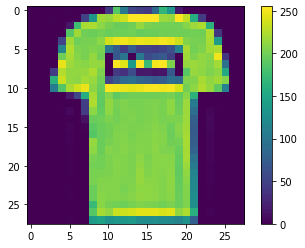

As you can see the image is a top and the value at index 1 of y_train also corresponds to the class name top.

y_train

array([9, 0, 0, ..., 3, 0, 5], dtype=uint8)

Neural Network model doesn't take value greater than 1. So we need to bring all the values between 0 and 1. To do this we will divide all the values in the training and testing dataset by 255 as the greatest value in our dataset is 255.

X_train = X_train/255.0
X_test = X_test/255.0

Now we can see that all the values are between 0 and 1.

plt.figure()
plt.imshow(X_train[1])
plt.colorbar()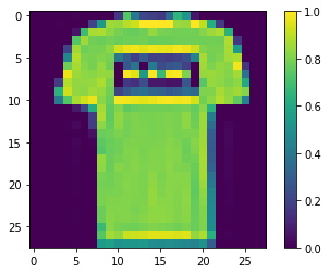

Build the model with TF 2.0

We will import the necessary layers to build the model.

The Neural Network is constructed from 3 type of layers:

• Input layer — initial data for the neural network.
• Hidden layers — intermediate layer between input and output layer and place where all the computation is done.
• Output layer — produce the result for given inputs.

from tensorflow.keras import Sequential
from tensorflow.keras.layers import Flatten, Dense

Flatten() is used as the input layer to convert the data into a 1-dimensional array for inputting it to the next layer. Our image 2D image will be converted to a single 1D column. input_shape = (28,28) because the size of our input image is 28x28.

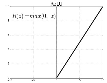
Dense() layer is the regular deeply connected neural network layer. It is most common and frequently used layer. We have a dense layer with 128 neurons with activation function relu. The rectified linear activation function or ReLU for short is a piecewise linear function that will output the input directly if it is positive, otherwise, it will output zero.

The output layer is a dense layer with 10 neurons because we have 10 classes. The activation function used is softmax. Softmax converts a real vector to a vector of categorical probabilities. The elements of the output vector are in range (0, 1) and sum to 1. Softmax is often used as the activation for the last layer of a classification network because the result could be interpreted as a probability distribution.

model = Sequential()
model.add(Flatten(input_shape = (28, 28)))
model.add(Dense(128, activation = 'relu'))
model.add(Dense(10, activation = 'softmax'))

model.summary()

Model: "sequential_1"
_________________________________________________________________
Layer (type)                 Output Shape              Param #
=================================================================
flatten_1 (Flatten)          (None, 784)               0
_________________________________________________________________
dense_2 (Dense)              (None, 128)               100480
_________________________________________________________________
dense_3 (Dense)              (None, 10)                1290
=================================================================
Total params: 101,770
Trainable params: 101,770
Non-trainable params: 0
_________________________________________________________________

Model compilation

• Loss Function: A loss function is used to optimize the parameter values in a neural network model. Loss functions map a set of parameter values for the network onto a scalar value that indicates how well those parameter accomplish the task the network is intended to do.
• Optimizer: Optimizers are algorithms or methods used to change the attributes of your neural network such as weights and learning rate in order to reduce the losses.
• Metrics: A metric is a function that is used to judge the performance of your model. Metric functions are similar to loss functions, except that the results from evaluating a metric are not used when training the model.

Here we are compiling the model and fitting it to the training data. We will use 10 epochs to train the model. An epoch is an iteration over the entire data provided.

model.compile(optimizer='adam', loss = 'sparse_categorical_crossentropy', metrics = ['accuracy'])
model.fit(X_train, y_train, epochs = 10)

Train on 60000 samples

Epoch 9/10
60000/60000 [==============================] - 5s 79us/sample - loss: 0.2472 - accuracy: 0.9081
Epoch 10/10
60000/60000 [==============================] - 5s 80us/sample - loss: 0.2374 - accuracy: 0.9120

Now we will evaluate the accuracy using the test data. We have got an accuracy of 88.41%.

test_loss, test_acc = model.evaluate(X_test, y_test)
print(test_acc)

10000/10000 [==============================] - 1s 81us/sample - loss: 0.3312 - accuracy: 0.8841
0.8841

Now we are going to do predictions using sklearn and see the accuracy. For that we will import accuracy_score from sklearn.

from sklearn.metrics import accuracy_score

predict_classes generates class predictions for the input samples. Here we are giving X_test containing 10000 images as the input. We are even predicting the accuracy. In multilabel classification, accuracy_score computes subset accuracy: the set of labels predicted for a sample must exactly match the corresponding set of labels in y_test.

y_pred = model.predict_classes(X_test)
accuracy_score(y_test, y_pred)

0.8841

Now we will use this model to perform predictions on an input image.

y_pred

array([9, 2, 1, ..., 8, 1, 5], dtype=int64)

predict() returns an array unlike predict_class() which returns categorical values. The array contains the confidence level for each of the class.

pred = model.predict(X_test)
pred

array([[2.3493649e-07, 1.7336136e-09, 3.9774801e-09, ..., 1.7785656e-03,
        3.6985359e-08, 9.9811894e-01],
       [7.2894422e-06, 5.1075269e-15, 9.9772221e-01, ..., 2.2120526e-12,
        6.0182694e-09, 2.4706193e-16],
       [1.3015335e-07, 9.9999988e-01, 3.9984838e-12, ..., 1.3045939e-23,
        3.1408490e-11, 2.1719039e-15],
       ...

As you can see for the test image at index 0, predict has retured this array. In this the value at index 9 is the greatest. This shows that the model has predicted the test image at index 0 to have class 9 which is ankle boot.

pred[0]

array([2.3493649e-07, 1.7336136e-09, 3.9774801e-09, 1.0847069e-08,
       2.9475926e-09, 1.0172284e-04, 3.8994517e-07, 1.7785656e-03,
       3.6985359e-08, 9.9811894e-01], dtype=float32)

argmax() returns the index of the maximum value. Hence we can see that the predicted class is 9 as maximum value is found at index position 9.

np.argmax(pred[0])

9

For the second image in the test data i.e. the image at index 1 the predicted class is 2 which is pullover.

np.argmax(pred[1])

2

The model gives an accuracy of 91.2% on the training data and 88.41% on test data. Hence the model is overfitting the training data. Overfitting happens when a model learns the detail and noise in the training data to the extent that it negatively impacts the performance of the model on new data. This means that the noise or random fluctuations in the training data is picked up and learned as concepts by the model. The problem is that these concepts do not apply to new data and negatively impact the models ability to generalize. To avoid overfitting we can use Convolutional Neural Networks.

Conclusion

In this tutorial you built and trained a fully connected ANN in TensorFlow 2.0 to classify Fashion MNIST images into 10 clothing categories. After normalizing pixel values to the 0–1 range, a three-layer model (Flatten → 128-neuron Dense → 10-neuron softmax) trained for 10 epochs reached 91.2% training accuracy and 88.41% test accuracy.

Key takeaways:

• Dividing image pixel values by 255 is the simplest normalization strategy — it maps all inputs to [0, 1] without fitting a scaler, which is sufficient for standard grayscale image datasets.
• A gap between training accuracy (91.2%) and test accuracy (88.4%) is a sign of mild overfitting — adding Dropout or switching to a CNN would close this gap.
• predict_classes() returns a single class index per sample; predict() returns the full softmax probability vector, which you can use with argmax() to get the same result.

Next steps:

• Replace the Dense layers with convolutional blocks in 2D CNN on CIFAR-10 to see how spatial feature learning improves accuracy.
• Build the same ANN from scratch on tabular data in Building Your First ANN with TensorFlow 2.0.
• Experiment with adding one or two Dropout(0.3) layers between the Dense blocks to reduce the overfitting gap.