Multi-Label Image Classification in Python
In this project, we are going to train our model on a set of labeled movie posters. The model will predict the genres of the movie based on the movie poster. We will consider a set of 25 genres. Each poster can have more than one genre.
Dataset
Dataset Link: https://www.cs.ccu.edu.tw/~wtchu/projects/MoviePoster/index.html
This dataset was collected from the IMDB website. One poster image was collected from one (mostly) Hollywood movie released from 1980 to 2015. Each poster image is associated with a movie as well as some metadata like ID, genres, and box office. The ID of each image is set as its file name.
You can even clone the github repository using the following command to get the dataset.
!git clone https://github.com/laxmimerit/Movies-Poster_Dataset.gitTensorflow Installation
We are going to use tensorflow to build the model. You can install tensorflow by running this command. If you machine has a GPU you can use the second command.
pip install tensorflow
pip install tensorflow-gpu
Watch Full Video Here:
import tensorflow as tf
from tensorflow.keras import Sequential
from tensorflow.keras.layers import Flatten, Dense, Dropout, BatchNormalization, Conv2D, MaxPool2D
from tensorflow.keras.optimizers import Adam
from tensorflow.keras.preprocessing import image
print(tf.__version__)2.1.0import numpy as np
import pandas as pd
import matplotlib.pyplot as plt
from sklearn.model_selection import train_test_split
from tqdm import tqdmHere we are reading the dataset into a pandas dataframe using pd.read_csv(). The dataset contains 7254 rows and 27 columns.
data = pd.read_csv('/content/Movies-Poster_Dataset/train.csv')
data.shape(7254, 27)data.head() shows the first 5 rows of the dataset. The dataset contains the Id of the image. The images are stored in a separate folder with the Id as the name of the image file.
data.head()| Id | Genre | Action | Adventure | Animation | Biography | Comedy | Crime | Documentary | Drama | Family | Fantasy | History | Horror | Music | Musical | Mystery | N/A | News | Reality-TV | Romance | Sci-Fi | Short | Sport | Thriller | War | Western | |
|---|---|---|---|---|---|---|---|---|---|---|---|---|---|---|---|---|---|---|---|---|---|---|---|---|---|---|---|
| 0 | tt0086425 | ['Comedy', 'Drama'] | 0 | 0 | 0 | 0 | 1 | 0 | 0 | 1 | 0 | 0 | 0 | 0 | 0 | 0 | 0 | 0 | 0 | 0 | 0 | 0 | 0 | 0 | 0 | 0 | 0 |
| 1 | tt0085549 | ['Drama', 'Romance', 'Music'] | 0 | 0 | 0 | 0 | 0 | 0 | 0 | 1 | 0 | 0 | 0 | 0 | 1 | 0 | 0 | 0 | 0 | 0 | 1 | 0 | 0 | 0 | 0 | 0 | 0 |
| 2 | tt0086465 | ['Comedy'] | 0 | 0 | 0 | 0 | 1 | 0 | 0 | 0 | 0 | 0 | 0 | 0 | 0 | 0 | 0 | 0 | 0 | 0 | 0 | 0 | 0 | 0 | 0 | 0 | 0 |
| 3 | tt0086567 | ['Sci-Fi', 'Thriller'] | 0 | 0 | 0 | 0 | 0 | 0 | 0 | 0 | 0 | 0 | 0 | 0 | 0 | 0 | 0 | 0 | 0 | 0 | 0 | 1 | 0 | 0 | 1 | 0 | 0 |
| 4 | tt0086034 | ['Action', 'Adventure', 'Thriller'] | 1 | 1 | 0 | 0 | 0 | 0 | 0 | 0 | 0 | 0 | 0 | 0 | 0 | 0 | 0 | 0 | 0 | 0 | 0 | 0 | 0 | 0 | 1 | 0 | 0 |
The images in the dataset are of different sizes. To process the images we need to convert them into a fixed size. tqdm() shows a progress bar while loading the images. We are going to loop through each image using its path. We are going to convert each image to a fixed size of 350x350. The values in the images are between 0 to 255. Neural networks work well with values between 0 to 1. Hence we are going to normalize the values by dividing all of the values by 255.
img_width = 350
img_height = 350

X = []

for i in tqdm(range(data.shape[0])):
  path = '/content/Movies-Poster_Dataset/Images/' + data['Id'][i] + '.jpg'
  img = image.load_img(path, target_size=(img_width, img_height, 3))
  img = image.img_to_array(img)
  img = img/255.0
  X.append(img)

X = np.array(X)100%|██████████| 7254/7254 [00:33<00:00, 216.79it/s]X is a numpy array which has 7254 images. Each image has the size 350x350 and is 3 dimensional as the image is a coloured image.
X.shape(7254, 350, 350, 3)Now we will see an image from X.
plt.imshow(X[1])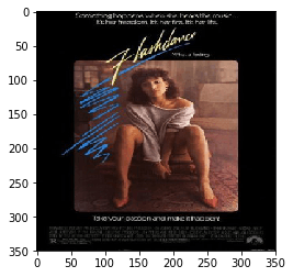
We can get the Genre of the above image from data.
data['Genre'][1]"['Drama', 'Romance', 'Music']"Now we will prepare the dataset. We have already got the feature space in X. Now we will get the target in y. For that, we will drop the Id and Genre columns from data.
y = data.drop(['Id', 'Genre'], axis = 1)
y = y.to_numpy()
y.shape(7254, 25)Now we will split the data into training and testing set with the help of train_test_split(). test_size = 0.15 will keep 15% data for testing and 85% data will be used for training the model. random_state controls the shuffling applied to the data before applying the split.
X_train, X_test, y_train, y_test = train_test_split(X, y, random_state = 0, test_size = 0.15)This is the input shape which we will pass as a para,eter to the first layer of our model.
X_train[0].shape(350, 350, 3)Build CNN
A Sequential() model is appropriate for a plain stack of layers where each layer has exactly one input tensor and one output tensor.
Conv2D is a 2D Convolution Layer, this layer creates a convolution kernel that is wind with layers input which helps produce a tensor of outputs. In the first Conv2D() layer we are learning a total of 16 filters with size of convolutional window as 3x3. The input_shape specifies the shape of the input. It is a necessary parameter for the first layer in any neural network. We will be using ReLu activation function. The rectified linear activation function or ReLU for short is a piecewise linear function that will output the input directly if it is positive, otherwise, it will output zero.
BatchNormalization() allows each layer of a network to learn by itself a little bit more independently of other layers. To increase the stability of a neural network, batch normalization normalizes the output of a previous activation layer by subtracting the batch mean and dividing by the batch standard deviation. It applies a transformation that maintains the mean output close to 0 and the output standard deviation close to 1.
MaxPool2D downsamples the input representation by taking the maximum value over the window defined by pool_size for each dimension along the features axis. The pool_size is 2x2 in our model.
Dropout() is used to randomly set the outgoing edges of hidden units to 0 at each update of the training phase. The value passed in dropout specifies the probability at which outputs of the layer are dropped out.
Flatten() is used to convert the data into a 1-dimensional array for inputting it to the next layer.
Dense() is the regular deeply connected neural network layer. The output layer is also a dense layer with 25 neurons because we are predicting a probability for 25 classes. Sigmoid function is used because it exists between (0 to 1) and this facilitates us to predict a binary output. Even though we are predicting more than one label, if you see in the target y all the values are either 0 or 1. Hence Sigmoid function is the appropriate function for this model.
model = Sequential()
model.add(Conv2D(16, (3,3), activation='relu', input_shape = X_train[0].shape))
model.add(BatchNormalization())
model.add(MaxPool2D(2,2))
model.add(Dropout(0.3))

model.add(Conv2D(32, (3,3), activation='relu'))
model.add(BatchNormalization())
model.add(MaxPool2D(2,2))
model.add(Dropout(0.3))

model.add(Conv2D(64, (3,3), activation='relu'))
model.add(BatchNormalization())
model.add(MaxPool2D(2,2))
model.add(Dropout(0.4))

model.add(Conv2D(128, (3,3), activation='relu'))
model.add(BatchNormalization())
model.add(MaxPool2D(2,2))
model.add(Dropout(0.5))

model.add(Flatten())

model.add(Dense(128, activation='relu'))
model.add(BatchNormalization())
model.add(Dropout(0.5))

model.add(Dense(128, activation='relu'))
model.add(BatchNormalization())
model.add(Dropout(0.5))

model.add(Dense(25, activation='sigmoid'))model.summary()Model: "sequential"
_________________________________________________________________
Layer (type) Output Shape Param #
=================================================================
conv2d (Conv2D) (None, 348, 348, 16) 448
_________________________________________________________________
batch_normalization (BatchNo (None, 348, 348, 16) 64
_________________________________________________________________
max_pooling2d (MaxPooling2D) (None, 174, 174, 16) 0
_________________________________________________________________
dropout (Dropout) (None, 174, 174, 16) 0
_________________________________________________________________
conv2d_1 (Conv2D) (None, 172, 172, 32) 4640
_________________________________________________________________
batch_normalization_1 (Batch (None, 172, 172, 32) 128
_________________________________________________________________
max_pooling2d_1 (MaxPooling2 (None, 86, 86, 32) 0
_________________________________________________________________
dropout_1 (Dropout) (None, 86, 86, 32) 0
_________________________________________________________________
conv2d_2 (Conv2D) (None, 84, 84, 64) 18496
_________________________________________________________________
batch_normalization_2 (Batch (None, 84, 84, 64) 256
_________________________________________________________________
max_pooling2d_2 (MaxPooling2 (None, 42, 42, 64) 0
_________________________________________________________________
dropout_2 (Dropout) (None, 42, 42, 64) 0
_________________________________________________________________
conv2d_3 (Conv2D) (None, 40, 40, 128) 73856
_________________________________________________________________
batch_normalization_3 (Batch (None, 40, 40, 128) 512
_________________________________________________________________
max_pooling2d_3 (MaxPooling2 (None, 20, 20, 128) 0
_________________________________________________________________
dropout_3 (Dropout) (None, 20, 20, 128) 0
_________________________________________________________________
flatten (Flatten) (None, 51200) 0
_________________________________________________________________
dense (Dense) (None, 128) 6553728
_________________________________________________________________
batch_normalization_4 (Batch (None, 128) 512
_________________________________________________________________
dropout_4 (Dropout) (None, 128) 0
_________________________________________________________________
dense_1 (Dense) (None, 128) 16512
_________________________________________________________________
batch_normalization_5 (Batch (None, 128) 512
_________________________________________________________________
dropout_5 (Dropout) (None, 128) 0
_________________________________________________________________
dense_2 (Dense) (None, 25) 3225
=================================================================
Total params: 6,672,889
Trainable params: 6,671,897
Non-trainable params: 992
_________________________________________________________________Now we will compile and fit the model. We will use 5 epochs to train the model. An epoch is an iteration over the entire data provided. validation_data is the data on which to evaluate the loss and any model metrics at the end of each epoch. As metrics = ['accuracy'] the model will be evaluated based on the accuracy.
model.compile(optimizer='adam', loss = 'binary_crossentropy', metrics=['accuracy'])
history = model.fit(X_train, y_train, epochs=5, validation_data=(X_test, y_test))Train on 6165 samples, validate on 1089 samples
Epoch 1/5
6165/6165 [==============================] - 720s 117ms/sample - loss: 0.6999 - accuracy: 0.6431 - val_loss: 0.5697 - val_accuracy: 0.7450
Epoch 2/5
6165/6165 [==============================] - 721s 117ms/sample - loss: 0.3138 - accuracy: 0.8869 - val_loss: 0.2531 - val_accuracy: 0.9071
Epoch 3/5
6165/6165 [==============================] - 718s 116ms/sample - loss: 0.2615 - accuracy: 0.9057 - val_loss: 0.2407 - val_accuracy: 0.9078
Epoch 4/5
6165/6165 [==============================] - 720s 117ms/sample - loss: 0.2525 - accuracy: 0.9085 - val_loss: 0.2388 - val_accuracy: 0.9096
Epoch 5/5
6165/6165 [==============================] - 723s 117ms/sample - loss: 0.2468 - accuracy: 0.9100 - val_loss: 0.2362 - val_accuracy: 0.9119Now we will visualize the results.
def plot_learningCurve(history, epoch):
  # Plot training & validation accuracy values
  epoch_range = range(1, epoch+1)
  plt.plot(epoch_range, history.history['accuracy'])
  plt.plot(epoch_range, history.history['val_accuracy'])
  plt.title('Model accuracy')
  plt.ylabel('Accuracy')
  plt.xlabel('Epoch')
  plt.legend(['Train', 'Val'], loc='upper left')
  plt.show()

  # Plot training & validation loss values
  plt.plot(epoch_range, history.history['loss'])
  plt.plot(epoch_range, history.history['val_loss'])
  plt.title('Model loss')
  plt.ylabel('Loss')
  plt.xlabel('Epoch')
  plt.legend(['Train', 'Val'], loc='upper left')
  plt.show()

plot_learningCurve(history, 5)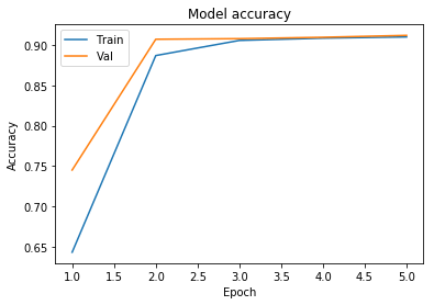
Training and validation loss decreased steadily together, confirming the model is not overfitting.
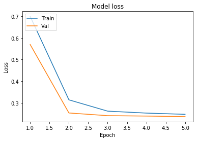
We can see that the validation accuracy is more than the training accuracy and the validation loss is less than the training loss. Hence the model is not overfitting.
Testing of model
Now we are going to test our model by giving it a new image. We will pre-process the image in the same way as we have pre-processed the images in the training and testing dataset. We will normalize them and convert them into a size of 350x350. classes contains all the 25 classes which we have considered. model.predict() will give us the probabilities for all the 25 classes. We will sort the probabilities using np.argsort() and then select the classes having the top 3 probabilities.
img = image.load_img('saaho.jpg', target_size=(img_width, img_height, 3))
plt.imshow(img)
img = image.img_to_array(img)
img = img/255.0

img = img.reshape(1, img_width, img_height, 3)

classes = data.columns[2:]
print(classes)
y_prob = model.predict(img)
top3 = np.argsort(y_prob[0])[:-4:-1]

for i in range(3):
print(classes[top3[i]])Index(['Action', 'Adventure', 'Animation', 'Biography', 'Comedy', 'Crime',
'Documentary', 'Drama', 'Family', 'Fantasy', 'History', 'Horror',
'Music', 'Musical', 'Mystery', 'N/A', 'News', 'Reality-TV', 'Romance',
'Sci-Fi', 'Short', 'Sport', 'Thriller', 'War', 'Western'],
dtype='object')
Drama
Action
Adventure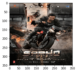
As you can see for the above movie poster our model has selected 3 genres which are Drama, Action and Adventure.
Conclusion
In this tutorial you built a multi-label movie genre classifier that assigns up to 25 genres to a movie poster using a 4-block Conv2D + BatchNorm + MaxPool CNN. Trained on 6,165 poster images and tested on 1,089, the model reached 91.2% validation accuracy in just 5 epochs, with training and validation curves tracking closely — confirming no overfitting. A live prediction on the Saaho poster correctly identified Drama, Action, and Adventure as the top-3 genres.
Key takeaways:
- Multi-label classification uses a sigmoid output layer (not softmax): each neuron independently outputs a probability for one genre, so a single image can activate multiple labels simultaneously.
- Binary cross-entropy is the correct loss for multi-label problems — it treats each of the 25 genre outputs as a separate binary prediction rather than enforcing a probability sum of 1.
BatchNormalization()after eachConv2Dblock stabilizes training by normalizing activations, allowing a deeper 4-block architecture to converge without exploding or vanishing gradients.- When validation accuracy consistently exceeds training accuracy (as seen here), the model is generalizing well — the difference is often due to Dropout being active only during training.
Next steps:
- Compare against a pre-trained backbone in Image Classification using Pre-trained VGG-16 to see how transfer learning handles small datasets.
- Try Hamming loss as an explicit multi-label evaluation metric to measure per-label accuracy rather than exact-match subset accuracy.
- Extend predictions to the top-5 genres and evaluate with mean average precision (mAP) for a more nuanced ranking metric.