We have spent this series inside a Transformer: tokens become vectors, attention connects positions, caches support generation, and GPU kernels carry out the work. This final lesson steps back. Before training a model, we must choose its size and decide how many data tokens it should see. A scaling law is an observed mathematical pattern that helps make that choice.
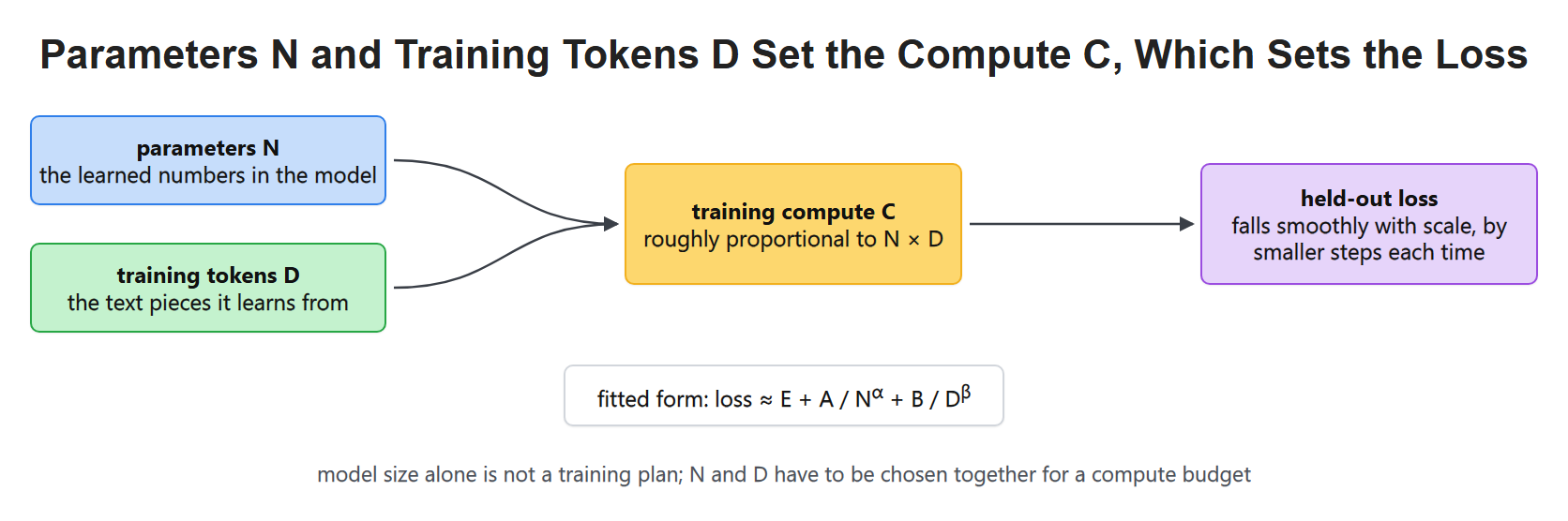
A training plan is a three-way balance, not a single choice of parameter count.
What Do We Measure?
Researchers often measure held-out loss, a number that tells us how surprised the model is by correct next tokens in text withheld from weight updates. Lower loss means the model assigns more probability to the text it should predict. Loss is not every aspect of model usefulness, but it is a clear training signal we can compare across planned runs.
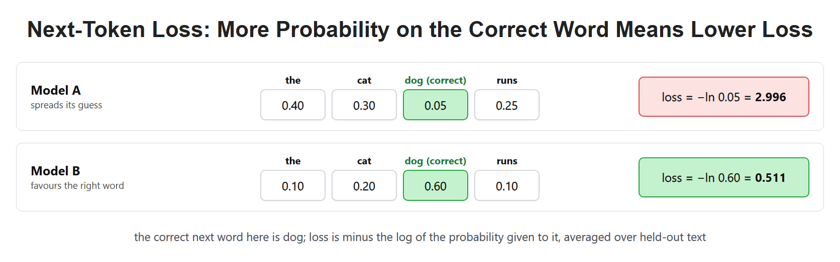
Loss gives a common ruler for comparing different training budgets.
As we add parameters, train on more tokens, or spend more compute, loss often falls in a smooth trend over a useful range. The improvement gets smaller as resources grow, so a ten-times-larger run does not usually make a ten-times-better model.
Three Knobs, One Budget
The main knobs are parameter count N, training-token count D, and training compute C. Parameters are the learned numbers in the model. Data tokens are the text pieces it trains on. Compute is the total arithmetic budget needed to train.
For a fixed architecture, training compute rises roughly with both parameter count and number of training tokens. A simplified planning relationship is C proportional to N x D. The real count includes details such as layers, sequence length, and optimizer work, but this relationship explains the trade-off.
What Does a Power Law Mean?
A simple fitted relationship can take the form:
$ \mathcal{L}(N,D)\approx E+\frac{A}{N^\alpha}+\frac{B}{D^\beta} $
is the predicted held-out loss. is a fitted lower-limit term. and set the sizes of the parameter-related and data-related contributions. Positive exponents and describe how quickly those contributions shrink as resources increase.
This is an empirical fit: researchers estimate its constants from training runs. It is not an exact identity for every model. If in a toy fit, multiplying parameters by four halves the parameter-related term, because . It does not halve the entire loss, since the other terms remain.
Controlled comparisons need the same evaluation data and compatible tokenization. A loss measured per token depends on how text is split. Changing tokenizers can change the unit being measured, making raw loss numbers misleading if compared without care.
A Model Can Be Undertrained
Suppose we choose an enormous model but give it too few training tokens. The model has many parameters but not enough examples to learn from them fully. Training ends because the compute budget has been spent, not because the model ran out of useful capacity.
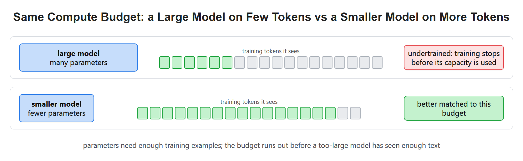
More parameters do not help as much when the training token budget stays small.
The opposite can also happen. A small model trained on a great deal of data may not have enough capacity to absorb all the patterns in that data. Planning is about avoiding either mismatch.
What Early Kaplan-Style Results Suggested
Early work by Kaplan and colleagues studied how loss changed with scale and argued for growing model size aggressively under a fixed compute budget. This influenced a period when training recipes often used very large models with comparatively fewer training tokens.
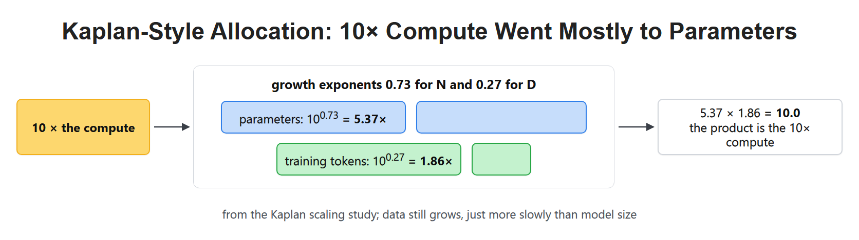
The best point depends on the empirical scaling relationship being used.
The key idea was not that data stopped mattering. It was that, under the measurements and assumptions of those studies, model size appeared to deserve a larger share of the fixed budget.
The Kaplan scaling study reported approximate compute-optimal growth exponents of 0.73 for parameters and 0.27 for training data. Here "compute-optimal" means the choice that gives the best measured loss for a fixed training arithmetic budget under the study's assumptions.
For ten times the compute, those exponents imply roughly times the parameters and times the training tokens. Their product is ten. The prescription was about how to allocate an increasing budget, not a claim that data could be ignored.
What Chinchilla Changed
Later Chinchilla results showed that many large language models were undertrained: they could benefit from substantially more data tokens for the same overall compute budget. The practical lesson was to balance model parameters and training tokens more evenly than several earlier recipes had done.
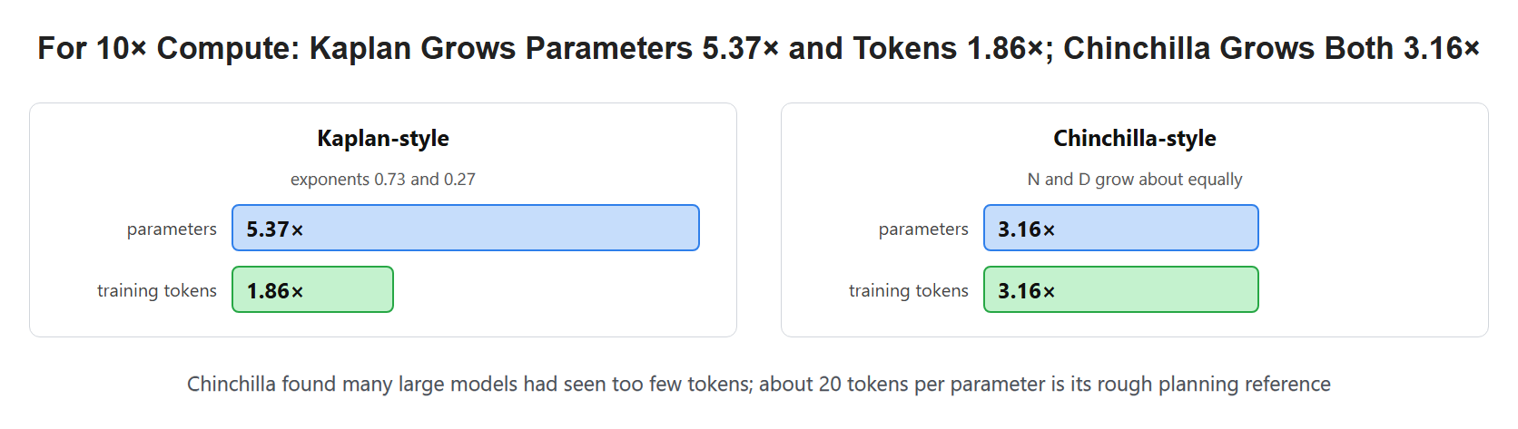
The newer recipe asks whether a large model has seen enough text, not only whether it has enough parameters.
A common rough rule from that result is around 20 training tokens per parameter for the studied setup. It is a planning reference, not a law of nature. Architecture, data quality, training goal, and changes in research can move the best ratio.
The Chinchilla study instead found that compute-optimal parameter count and token count should grow approximately together over its studied range. Under the simple equal-exponent picture, ten times the compute allows about times each.
Compare the two recipes using the same starting point, rather than treating either as a universal command. The important difference is the allocation of additional compute between more parameters and more training tokens.
Training-token count means processed tokens, not necessarily unique tokens. Repeating a dataset increases the processed count but does not supply the same diversity as new suitable text. That limits how literally we should interpret a token-count target when data is scarce.
A 70B-Parameter Thought Experiment
Using the rough 20-to-1 reference, a 70-billion-parameter model would train on about 1.4 trillion tokens:
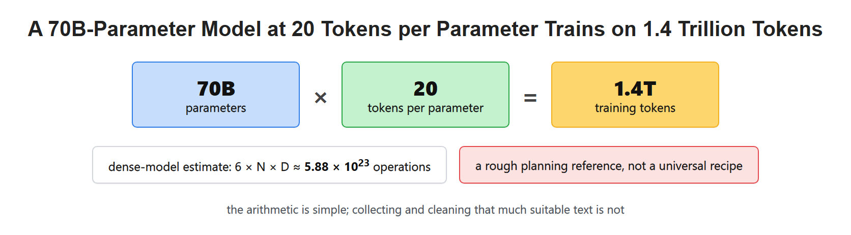
The arithmetic is simple; collecting and cleaning that much data is not.
We should not read this as an instruction to train a 70B model. It shows why parameter count alone is incomplete. The data plan can be as large a project as the model plan.
Check a Dense-Model Compute Estimate
A common rough estimate for dense Transformer training is floating-point operations. An operation is one arithmetic step such as an addition or multiplication. This planning estimate counts dominant parameter-related forward and backward work; it is not a complete hardware-time formula.
We use Python integers so the large counts remain exact until the final display conversion.
parameters = 70_000_000_000
tokens_per_parameter = 20
training_tokens = parameters * tokens_per_parameter
estimated_flops = 6 * parameters * training_tokens
This gives 1.4 trillion training tokens and about estimated operations. The factor six is an approximation, not a configurable training parameter. Sequence-length-dependent attention work, architecture details, optimizer work, communication, and hardware efficiency can change the actual cost.
A sparse mixture-of-experts model routes tokens through selected subnetworks rather than using every parameter each time. For that design, total stored parameters and active compute parameters differ. Do not apply a dense-model estimate blindly using its total parameter count.
Data Quality Is Not Just a Token Count
Two trillion repeated, noisy, or badly matched tokens are not equal to two trillion carefully selected, diverse tokens. Scaling-law equations make quantities easier to reason about, but they do not replace data filtering, deduplication, domain coverage, licensing checks, or evaluation.
This is especially important for a focused model. A code model, medical helper, or multilingual system needs data that matches the work we expect it to do.
Training Cost and Use-Time Cost Differ
More parameters usually mean more training compute and more memory at inference. More training data increases the training run but does not directly increase the parameter memory of a finished model. Long context adds another use-time cost through the KV cache we studied in Days 21 to 28.
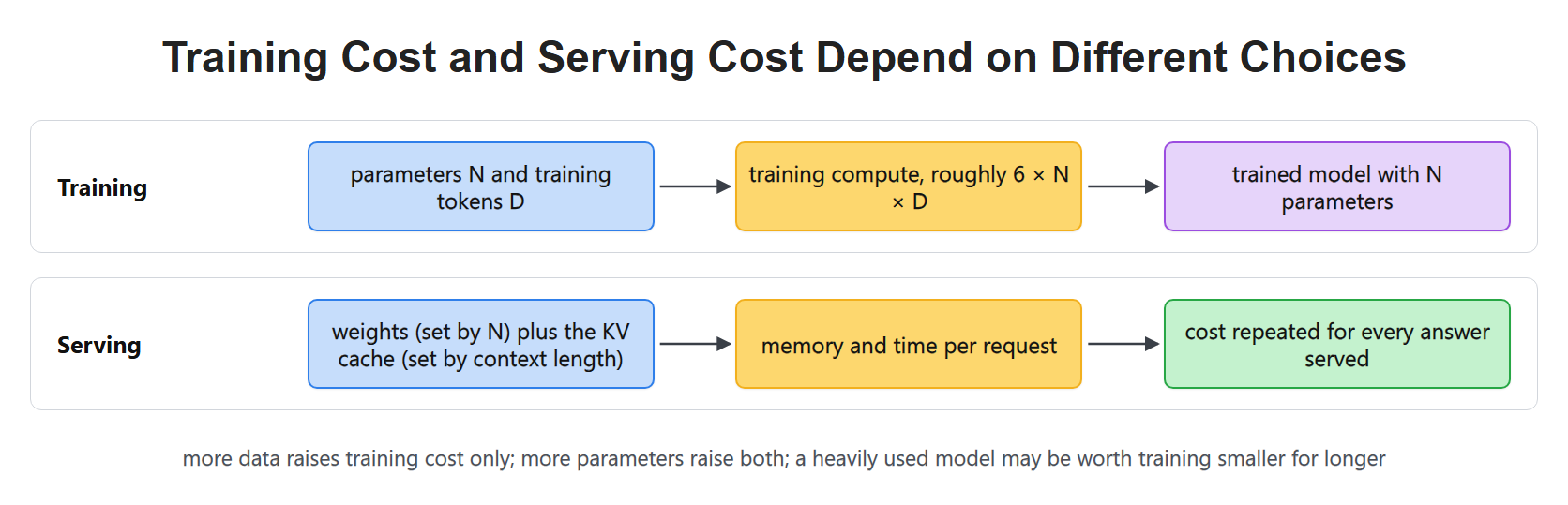
Parameter count affects both phases; data scale mainly affects training; context affects live cache memory.
The best recipe depends on the actual goal. A research team may optimize training loss under a fixed compute budget. A product team may also need to consider serving cost, response speed, privacy, and the kind of data it can legally use.
A training-compute optimum is not necessarily a lifetime-cost optimum. If a model will answer a very large number of requests, training a smaller model for longer can be worthwhile even when it departs from a training-only optimum. The finished model may cost less to run for every future answer. That decision needs a workload and quality target, not only a tokens-per-parameter rule.
To make a small research plan, train several sizes under controlled data and evaluation settings, record loss against processed tokens, fit candidate trends, and reserve additional runs to test those predictions. Extrapolating far beyond measured runs carries uncertainty. A fitted curve should guide a testable plan, not replace one.
Can We Teach the Architecture Back?
Before calling the series mastered, work through these checks without looking at a diagram. Name the input and output at every step, then compare your drawing with Day 19.
- Trace one token ID through embedding, position handling, a full attention-plus-MLP block, and the vocabulary output head.
- Calculate a three-key attention row, including scaling, a blocked future key, softmax, and the weighted values.
- Explain why the diagonal is allowed when training labels are shifted by one position.
- Show where the source enters an encoder-decoder model, and why cross-attention is rectangular.
- Draw the boundary between a selected output token and the cache entries created on its next forward pass.
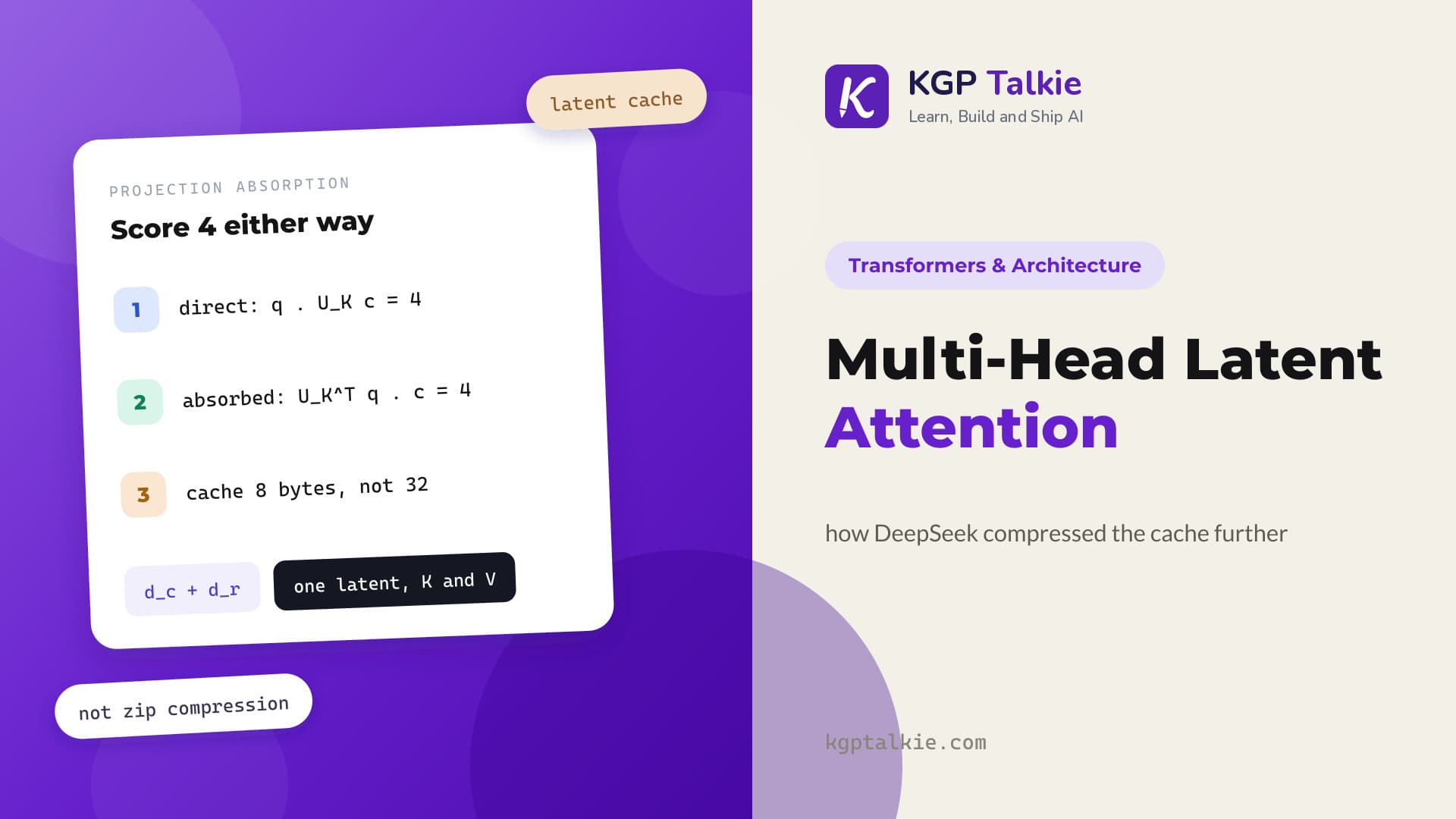
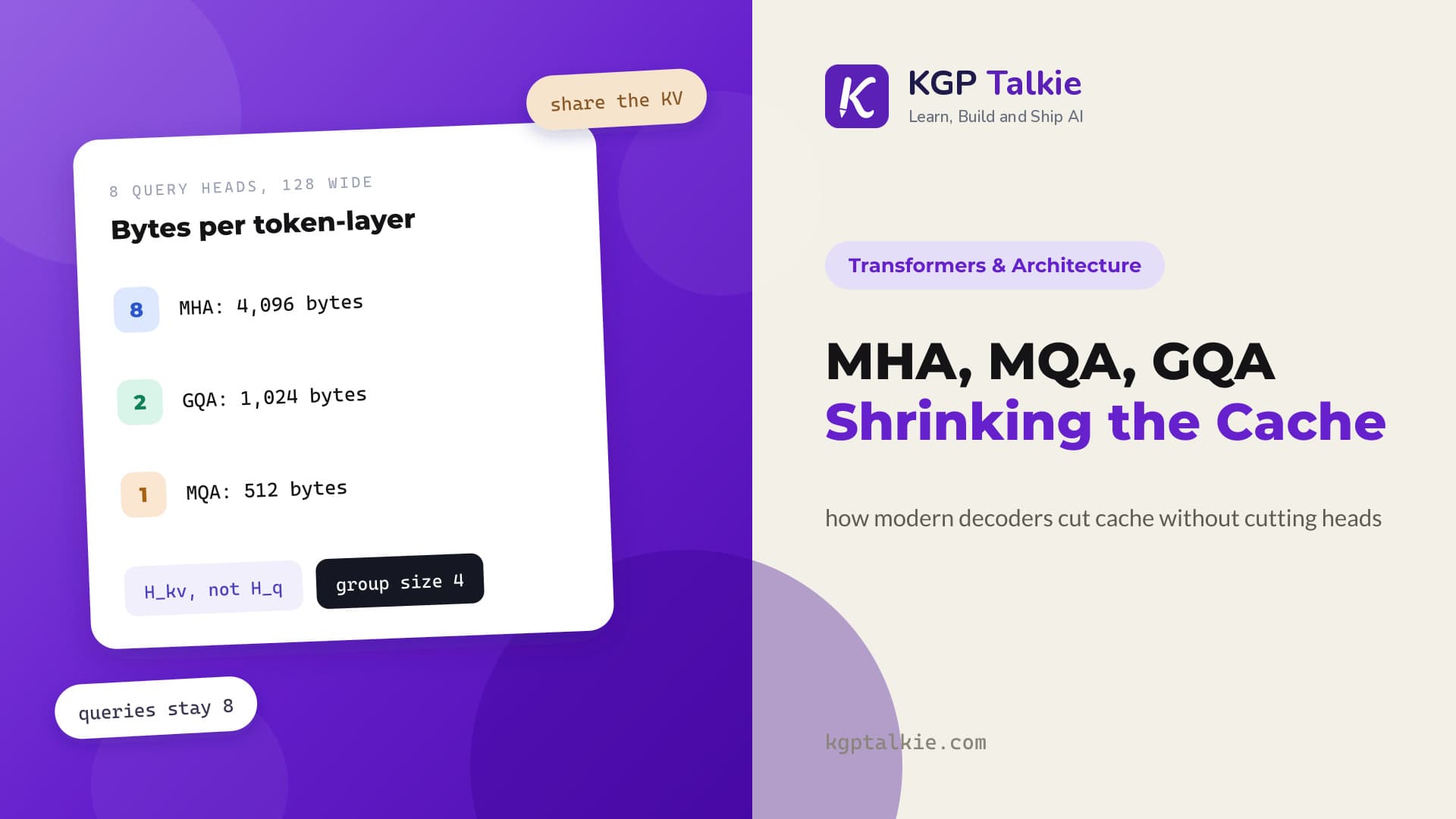
- Count a cache in bytes, then explain what changes under GQA, MLA, and paged storage.
- Explain which work FlashAttention avoids and which dense attention comparisons remain.
- Compare a parameter-heavy training plan with a more data-heavy plan at the same approximate compute.
These are teaching checks, not a guarantee that reading alone creates expertise. Being able to explain the diagrams, change the numbers correctly, and debug a wrong mask is better evidence of understanding than finishing thirty pages.
Recap: The Whole Series in One Map
Before we close, here is the full beginner map in words. Text is split into tokens. Token IDs become embeddings, and position information tells the model where each token sits. In a pre-norm layout, a Transformer block normalizes each token vector, uses attention to gather allowed context, adds that result through a residual connection, normalizes again, uses an MLP to change the representation at each position, and adds that result through another residual connection. The model repeats this block through many layers.
For an encoder, self-attention can use the complete input. For a decoder, causal attention hides future positions. An encoder-decoder model gives the decoder a cross-attention path to the encoder output. At the end of a decoder, an output head turns the newest hidden vector into vocabulary logits; softmax turns them into probabilities; a decoding rule chooses the next token. During training, shifted next-token labels and cross-entropy loss teach the weights. During use, a KV cache saves old attention information so the token-by-token loop does not recompute the full past.
This is how Transformer design connects from input to scale. Text becomes tokens, tokens become embeddings, attention uses Q, K, V plus position, residual and MLP layers build deeper representations, decoder caches make generation practical, and training choices balance parameters, data, and compute. Each decision changes what the model can learn or how it runs.
Scaling laws do not give a single permanent recipe. They give an evidence-based way to ask better planning questions: Is this model too large for its data? Are we spending compute where it helps most? What will the trained model cost to serve?
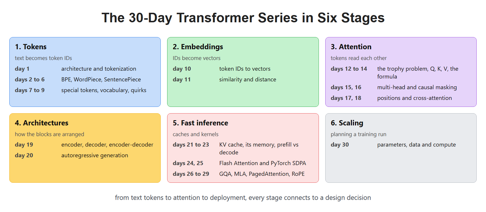
From text tokens to attention to deployment, every layer of the series connects to a design decision.