Feature Selection and CNN
In this project we are going to build a neural network to predict if a particular bank customer is satisfies or not. To do this we are going to use Convolutional Neural Networks. The dataset which we are going to use contains 370 features. Install TensorFlow with pip install tensorflow (or pip install tensorflow-gpu for GPU).
import numpy as np
import pandas as pd
import seaborn as sns
import matplotlib.pyplot as plt

from sklearn.model_selection import train_test_split
from sklearn.preprocessing import StandardScaler
from sklearn.feature_selection import VarianceThreshold

import tensorflow as tf
from tensorflow.keras import Sequential
from tensorflow.keras.layers import Conv1D, MaxPool1D, Flatten, Dense, Dropout, BatchNormalization
from tensorflow.keras.optimizers import Adam
print(tf.__version__)2.1.0You can use this command to directly get the data from github.
!git clone https://github.com/laxmimerit/Data-Files-for-Feature-Selection.gitAfter downloading the data, we will now read the data using read_csv(). To see the first 5 rows of the data we can use data.head().
data = pd.read_csv('train.csv')
data.head()| ID | var3 | var15 | imp_ent_var16_ult1 | imp_op_var39_comer_ult1 | imp_op_var39_comer_ult3 | imp_op_var40_comer_ult1 | imp_op_var40_comer_ult3 | imp_op_var40_efect_ult1 | imp_op_var40_efect_ult3 | ... | saldo_medio_var33_hace2 | saldo_medio_var33_hace3 | saldo_medio_var33_ult1 | saldo_medio_var33_ult3 | saldo_medio_var44_hace2 | saldo_medio_var44_hace3 | saldo_medio_var44_ult1 | saldo_medio_var44_ult3 | var38 | TARGET | |
|---|---|---|---|---|---|---|---|---|---|---|---|---|---|---|---|---|---|---|---|---|---|
| 0 | 1 | 2 | 23 | 0.0 | 0.0 | 0.0 | 0.0 | 0.0 | 0.0 | 0.0 | ... | 0.0 | 0.0 | 0.0 | 0.0 | 0.0 | 0.0 | 0.0 | 0.0 | 39205.170000 | 0 |
| 1 | 3 | 2 | 34 | 0.0 | 0.0 | 0.0 | 0.0 | 0.0 | 0.0 | 0.0 | ... | 0.0 | 0.0 | 0.0 | 0.0 | 0.0 | 0.0 | 0.0 | 0.0 | 49278.030000 | 0 |
| 2 | 4 | 2 | 23 | 0.0 | 0.0 | 0.0 | 0.0 | 0.0 | 0.0 | 0.0 | ... | 0.0 | 0.0 | 0.0 | 0.0 | 0.0 | 0.0 | 0.0 | 0.0 | 67333.770000 | 0 |
| 3 | 8 | 2 | 37 | 0.0 | 195.0 | 195.0 | 0.0 | 0.0 | 0.0 | 0.0 | ... | 0.0 | 0.0 | 0.0 | 0.0 | 0.0 | 0.0 | 0.0 | 0.0 | 64007.970000 | 0 |
| 4 | 10 | 2 | 39 | 0.0 | 0.0 | 0.0 | 0.0 | 0.0 | 0.0 | 0.0 | ... | 0.0 | 0.0 | 0.0 | 0.0 | 0.0 | 0.0 | 0.0 | 0.0 | 117310.979016 | 0 |
5 rows × 371 columns
We have 76020 rows in the dataset and 371 columns.
data.shape(76020, 371)Now we are going to create a feature space X. Feature space will only contain the column which provide information necessary for prediction. ID and TARGET do not play any role in prediction, so we are going to remove them using drop(). After droppring the 2 columns you can see that the number of columns have reduced to 369.
X = data.drop(labels=['ID', 'TARGET'], axis = 1)
X.shape(76020, 369)Lets create a variable y which contains the values which have to be predicted i.e. TARGET.
y = data['TARGET']Now we will split the data into training and testing set with the help of train_test_split(). test_size = 0.2 will keep 20% data for testing and 80% data will be used for training the model. random_state controls the shuffling applied to the data before applying the split. stratify = y means that the data is split in a stratified fashion, using y as the class labels.
X_train, X_test, y_train, y_test = train_test_split(X,y, test_size = 0.2, random_state = 0, stratify = y)As we can see, the training dataset consists of 60816 rows i.e. 80% of the data and the testing dataset consists of 15204 rows i.e 20% of the data.
X_train.shape, X_test.shape((60816, 369), (15204, 369))Remove Constant, Quasi Constant and Duplicate Features
Feature selection is the process of reducing the number of input variables when developing a predictive model.
Constant Featuresare the features that show single values in all the observations in the dataset. These features provide no information that allows ML models to predict the target.Quasi constantfeatures, as the name suggests, are the features that are almost constant. In other words, these features have the same values for a very large subset of the outputs. They have less variance. Such features are not very useful for making predictions.Duplicate Featuresas the name suggests are duplicated in the dataset.
Here we have set the variance threshold to 1% i.e. if any column has variance less than 1% it will be removed. In other words only the columns having variance greater than 99% will be retained. We are fitting VarianceThreshold() to the training data and not the test data. We are only transforming the test data.
filter = VarianceThreshold(0.01)
X_train = filter.fit_transform(X_train)
X_test = filter.transform(X_test)

X_train.shape, X_test.shape((60816, 273), (15204, 273))After removing the Quasi constant features we can see that 96 features are removed from the dataset.
369-27396Now we will remove the duplicate features. We don't have any direct function to remove duplicate features but we have functions to check for duplicate rows. Hence we are taking transpose of the data set using .T. As we can see after taking transpose the shape of X_train_T is exactly opposite to that of X_train.
X_train_T = X_train.T
X_test_T = X_test.T

X_train_T = pd.DataFrame(X_train_T)
X_test_T = pd.DataFrame(X_test_T)

X_train_T.shape(273, 60816).duplicated() returns a boolean Series denoting duplicate rows. We can see that 17 features are duplicated.
X_train_T.duplicated().sum()17Now we will see the list of dupicated features. The features having index True are duplicated.
duplicated_features = X_train_T.duplicated()
duplicated_features[70:90]70 False
71 False
72 True
73 False
74 True
75 False
76 False
77 False
78 False
79 False
80 False
81 False
82 False
83 False
84 False
85 False
86 False
87 False
88 False
89 False
dtype: boolWe have to retain the features with False value because they are not duplicated. So here we are going to use inversion i.e. we are going to change the False value to True and viceversa.
features_to_keep = [not index for index in duplicated_features]
features_to_keep[70:90][True, True, False, True, False, True, True, True, True, True, True, True, True, True, True, True, True, True, True, True]Now as we have inverted the values, we have to retain the features with value True. We also have to take transpose once again to get the data back in original shape. Here we have done it for X_train.
X_train = X_train_T[features_to_keep].T
X_train.shape(60816, 256)Here we have done it for X_test.
X_test = X_test_T[features_to_keep].T
X_test.shape(15204, 256)X_train.head()| 0 | 1 | 2 | 3 | 4 | 5 | 6 | 7 | 8 | 9 | ... | 263 | 264 | 265 | 266 | 267 | 268 | 269 | 270 | 271 | 272 | |
|---|---|---|---|---|---|---|---|---|---|---|---|---|---|---|---|---|---|---|---|---|---|
| 0 | 2.0 | 26.0 | 0.0 | 0.0 | 0.0 | 0.0 | 0.0 | 0.0 | 0.0 | 0.0 | ... | 0.0 | 0.0 | 0.0 | 0.0 | 0.0 | 0.0 | 0.0 | 0.0 | 0.0 | 117310.979016 |
| 1 | 2.0 | 23.0 | 0.0 | 0.0 | 0.0 | 0.0 | 0.0 | 0.0 | 0.0 | 0.0 | ... | 0.0 | 0.0 | 0.0 | 0.0 | 0.0 | 0.0 | 0.0 | 0.0 | 0.0 | 85472.340000 |
| 2 | 2.0 | 23.0 | 0.0 | 0.0 | 0.0 | 0.0 | 0.0 | 0.0 | 0.0 | 0.0 | ... | 0.0 | 0.0 | 0.0 | 0.0 | 0.0 | 0.0 | 0.0 | 0.0 | 0.0 | 317769.240000 |
| 3 | 2.0 | 30.0 | 0.0 | 0.0 | 0.0 | 0.0 | 0.0 | 0.0 | 0.0 | 0.0 | ... | 0.0 | 0.0 | 0.0 | 0.0 | 0.0 | 0.0 | 0.0 | 0.0 | 0.0 | 76209.960000 |
| 4 | 2.0 | 23.0 | 0.0 | 0.0 | 0.0 | 0.0 | 0.0 | 0.0 | 0.0 | 0.0 | ... | 0.0 | 0.0 | 0.0 | 0.0 | 0.0 | 0.0 | 0.0 | 0.0 | 0.0 | 302754.000000 |
5 rows × 256 columns
Now we are going to get the bring the data into the same range. StandardScaler() standardizes the features by removing the mean and scaling to unit variance.
scaler = StandardScaler()
X_train = scaler.fit_transform(X_train)
X_test = scaler.transform(X_test)
X_trainarray([[ 3.80478472e-02, -5.56029626e-01, -5.27331414e-02, ...,
-1.87046327e-02, -1.97720391e-02, 3.12133758e-03],
[ 3.80478472e-02, -7.87181903e-01, -5.27331414e-02, ...,
-1.87046327e-02, -1.97720391e-02, -1.83006062e-01],
[ 3.80478472e-02, -7.87181903e-01, -5.27331414e-02, ...,
-1.87046327e-02, -1.97720391e-02, 1.17499225e+00],
...,
[ 3.80478472e-02, 5.99731758e-01, -5.27331414e-02, ...,
-1.87046327e-02, -1.97720391e-02, -2.41865113e-01],
[ 3.80478472e-02, -1.70775831e-01, -5.27331414e-02, ...,
-1.87046327e-02, -1.97720391e-02, 3.12133758e-03],
[ 3.80478472e-02, 2.91528722e-01, 7.65192053e+00, ...,
-1.87046327e-02, -1.97720391e-02, 3.12133758e-03]])X_train.shape, X_test.shape((60816, 256), (15204, 256))Our data is 2 dimensional but neural networks accept 3 dimensional data. So we have to reshape() the data.
X_train = X_train.reshape(60816, 256,1)
X_test = X_test.reshape(15204, 256, 1)
X_train.shape, X_test.shape((60816, 256, 1), (15204, 256, 1))y_train = y_train.to_numpy()
y_test = y_test.to_numpy()Building the CNN
A Sequential() model is appropriate for a plain stack of layers where each layer has exactly one input tensor and one output tensor.
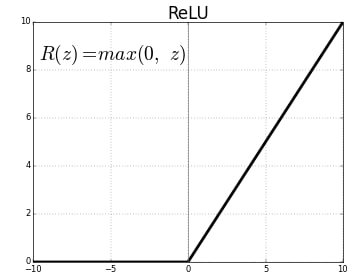
Conv1D() is a 1D Convolution Layer, this layer is very effective for deriving features from a fixed-length segment of the overall dataset, where it is not so important where the feature is located in the segment. In the first Conv1D() layer, we are learning a total of 36 filters with size of the convolutional window as 3. The input_shape specifies the shape of the input. It is a necessary parameter for the first layer in any neural network. We will be using the ReLu activation function. The rectified linear activation function or ReLU for short is a piecewise linear function that will output the input directly if it is positive, otherwise, it will output zero.
BatchNormalization() allows each layer of a network to learn by itself a little bit more independently of other layers. To increase the stability of a neural network, batch normalization normalizes the output of a previous activation layer by subtracting the batch mean and dividing by the batch standard deviation. It applies a transformation that maintains the mean output close to 0 and the output standard deviation close to 1.
MaxPool1D() downsamples the input representation by taking the maximum value over the window defined by pool_size which is 2 in case of the first Max Pool layer of this neural network.
Dropout() is used to randomly set the outgoing edges of hidden units to 0 at each update of the training phase. The value passed in dropout specifies the probability at which outputs of the layer are dropped out.
Flatten() is used to convert the data into a 1-dimensional array for inputting it to the next layer.
Dense() is the regular deeply connected neural network layer. The output layer is a dense layer with 1 neuron because we are predicting a single value. Sigmoid function is used because it exists between (0 to 1) and this facilitates us to predict a binary input.
model = Sequential()
model.add(Conv1D(32, 3, activation='relu', input_shape = (256,1)))
model.add(BatchNormalization())
model.add(MaxPool1D(2))
model.add(Dropout(0.3))

model.add(Conv1D(64, 3, activation='relu'))
model.add(BatchNormalization())
model.add(MaxPool1D(2))
model.add(Dropout(0.5))

model.add(Conv1D(128, 3, activation='relu'))
model.add(BatchNormalization())
model.add(MaxPool1D(2))
model.add(Dropout(0.5))

model.add(Flatten())
model.add(Dense(256, activation='relu'))
model.add(Dropout(0.5))

model.add(Dense(1, activation='sigmoid'))model.summary()Model: "sequential"
_________________________________________________________________
Layer (type) Output Shape Param #
=================================================================
conv1d (Conv1D) (None, 254, 32) 128
_________________________________________________________________
batch_normalization (BatchNo (None, 254, 32) 128
_________________________________________________________________
max_pooling1d (MaxPooling1D) (None, 127, 32) 0
_________________________________________________________________
dropout (Dropout) (None, 127, 32) 0
_________________________________________________________________
conv1d_1 (Conv1D) (None, 125, 64) 6208
_________________________________________________________________
batch_normalization_1 (Batch (None, 125, 64) 256
_________________________________________________________________
max_pooling1d_1 (MaxPooling1 (None, 62, 64) 0
_________________________________________________________________
dropout_1 (Dropout) (None, 62, 64) 0
_________________________________________________________________
conv1d_2 (Conv1D) (None, 60, 128) 24704
_________________________________________________________________
batch_normalization_2 (Batch (None, 60, 128) 512
_________________________________________________________________
max_pooling1d_2 (MaxPooling1 (None, 30, 128) 0
_________________________________________________________________
dropout_2 (Dropout) (None, 30, 128) 0
_________________________________________________________________
flatten (Flatten) (None, 3840) 0
_________________________________________________________________
dense (Dense) (None, 256) 983296
_________________________________________________________________
dropout_3 (Dropout) (None, 256) 0
_________________________________________________________________
dense_1 (Dense) (None, 1) 257
=================================================================
Total params: 1,015,489
Trainable params: 1,015,041
Non-trainable params: 448
_________________________________________________________________Now we will compile and fit the model. We are using Adam optimizer with 0.00005 learning rate. We will use 10 epochs to train the model. An epoch is an iteration over the entire data provided. validation_data is the data on which to evaluate the loss and any model metrics at the end of each epoch. The model will not be trained on this data. As metrics = ['accuracy'] the model will be evaluated based on the accuracy.
model.compile(optimizer=Adam(lr=0.00005), loss='binary_crossentropy', metrics=['accuracy'])
history = model.fit(X_train, y_train, epochs=10, validation_data=(X_test, y_test), verbose=1)Train on 60816 samples, validate on 15204 samples
Epoch 5/10
60816/60816 [==============================] - 111s 2ms/sample - loss: 0.1630 - accuracy: 0.9604 - val_loss: 0.1641 - val_accuracy: 0.9605
Epoch 6/10
60816/60816 [==============================] - 111s 2ms/sample - loss: 0.1599 - accuracy: 0.9603 - val_loss: 0.1595 - val_accuracy: 0.9605
Epoch 7/10
60816/60816 [==============================] - 111s 2ms/sample - loss: 0.1576 - accuracy: 0.9604 - val_loss: 0.1590 - val_accuracy: 0.9604
Epoch 8/10
60816/60816 [==============================] - 111s 2ms/sample - loss: 0.1556 - accuracy: 0.9604 - val_loss: 0.1610 - val_accuracy: 0.9605
Epoch 9/10
60816/60816 [==============================] - 111s 2ms/sample - loss: 0.1536 - accuracy: 0.9604 - val_loss: 0.1558 - val_accuracy: 0.9603
Epoch 10/10
60816/60816 [==============================] - 111s 2ms/sample - loss: 0.1542 - accuracy: 0.9604 - val_loss: 0.1602 - val_accuracy: 0.9599history gives us the summary of all the accuracies and losses calculated after each epoch.
history.history{'accuracy': [0.95417327, 0.9592706, 0.95992833, 0.96033937, 0.96037227, 0.9603065, 0.9604052, 0.960438, 0.9603887, 0.9604052], 'loss': [0.21693714527215763, 0.17656464240582592, 0.16882949567384484, 0.16588703954582057, 0.16303560407957227, 0.15994301885150822, 0.15763013028843298, 0.15563193596928912, 0.1535658989747522, 0.1542411554370529], 'val_accuracy': [0.9600763, 0.9600763, 0.96033937, 0.9604052, 0.9604709, 0.9604709, 0.9604052, 0.9604709, 0.9602736, 0.959879], 'val_loss': [0.17092196812710614, 0.1765108920851371, 0.16735200087523436, 0.1662461552617033, 0.16413307644895303, 0.1594827836499469, 0.15897791552088097, 0.16101698756464938, 0.15578439738331923, 0.16016060526129197]}We will now plot the model accuracy and model loss. In model accuracy we will plot the training accuracy and validation accuracy and in model loss we will plot the training loss and validation loss.
def plot_learningCurve(history, epoch):
  # Plot training & validation accuracy values
  epoch_range = range(1, epoch+1)
  plt.plot(epoch_range, history.history['accuracy'])
  plt.plot(epoch_range, history.history['val_accuracy'])
  plt.title('Model accuracy')
  plt.ylabel('Accuracy')
  plt.xlabel('Epoch')
  plt.legend(['Train', 'Val'], loc='upper left')
  plt.show()

  # Plot training & validation loss values
  plt.plot(epoch_range, history.history['loss'])
  plt.plot(epoch_range, history.history['val_loss'])
  plt.title('Model loss')
  plt.ylabel('Loss')
  plt.xlabel('Epoch')
  plt.legend(['Train', 'Val'], loc='upper left')
  plt.show()

plot_learningCurve(history, 10)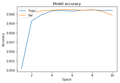
The loss plot confirms the same trend — both curves fall steadily with no sign of divergence:
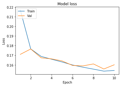
We have got an accuracy of 96%. Hence we can conclude that Convolutional neural networks with appropriate feature selection can build a very powerful model for this dataset. Feature selection enables the machine learning algorithm to train faster. It reduces the complexity of a model and makes it easier to interpret. It also improves the accuracy of a model if the right subset is chosen.
Conclusion
In this tutorial you built a 1D CNN to predict bank customer satisfaction from 370 raw features. After removing constant, quasi-constant, and duplicate features, the dataset shrank to 256 informative columns. Trained on 60,816 samples for 10 epochs, the model achieved ~96% accuracy on the held-out test set, with training and validation curves tracking closely throughout.
Key takeaways:
- Feature selection (variance thresholding and duplicate removal) cut 370 features to 256 without sacrificing predictive power — smaller inputs mean faster training and less overfitting risk.
- 1D CNNs can classify structured tabular data by treating each feature as a channel in a sequence; you do not need recurrent layers for this task.
StandardScaleris essential before feeding tabular data to a CNN — unnormalized large-magnitude features would dominate the convolutional filters.
Next steps:
- Apply the same 1D CNN approach to IMDB Sentiment Classification to see how convolutional filters work on text sequences.
- Try Human Activity Recognition with Accelerometer Data for another 1D sequence classification problem.
- Experiment with adding more convolutional blocks or a higher learning rate schedule to push accuracy above 96%.