IMDB Sentiment Classification with LSTM

Sentiment Classification in Python

Long Short-Term Memory (LSTM) networks handle long-range dependencies in text sequences through gated memory cells — making them well-suited for sentiment analysis. This tutorial builds an LSTM classifier with a trainable Embedding layer on the IMDB movie reviews dataset for binary positive/negative sentiment prediction.

Dataset

The IMDB dataset contains 50,000 movie reviews for natural language processing or Text analytics. It has two columns-review and sentiment. The review contains the actual review and the sentiment tells us whether the review is positive or negative. You can find the dataset here IMDB Dataset

Instead of downloading the dataset we will be directly using the IMDB dataset provided by keras.This is a dataset of 25,000 movies reviews for training and testing each from IMDB, labeled by sentiment (positive/negative). Reviews have been preprocessed, and each review is encoded as a list of word indexes (integers). For convenience, words are indexed by overall frequency in the dataset, so that for instance the integer "3" encodes the 3rd most frequent word in the data.

This will install a new version of tensorflow

!pip install tensorflow-gpu

Word to Vector

Computers do not understand human language. They require numbers to perform any sort of job. Hence in NLP, all the data has to be converted to numerical form before processing.

• As given in the diagram the sentence is first split into words.
• Then a vocabluary is created of the words in the entire data set.
• Then the words are encoded using a sparse matrix.
• Sparse matrix is a matrix in which most of the elements are 0.
• In this notebook we are going to use a dense matrix.
• It is a matrix where majority of the elements are non-zero.
• The IMDB dataset from Keras is already encoded using a dense matrix.

import numpy as np
import matplotlib.pyplot as plt
import tensorflow as tf

from tensorflow.keras.datasets import imdb
from tensorflow.keras.preprocessing.sequence import pad_sequences

This is used to check the tensorflow version

tf.__version__

Dataset preprocessing

imdb.load_data() returns a Tuple of Numpy arrays for training and testing: (x_train, y_train), (x_test, y_test) x_train, x_test: lists of sequences, which are lists of indexes (integers) y_train, y_test: lists of integer labels (1 or 0)

We have set num_words to 20000. Hence only 20000 most frequent words are kept. The maximum possible index value is num_words - 1

(X_train, y_train), (X_test, y_test) = imdb.load_data(num_words = 20000)

Here we can see that X_train is an array of lists where each list represents a review. We can see that the lengths of each review is different.

X_train[0][:5]

array([1415,   33,    6,   22,   12])

The length of all the reviews must be same before feeding them to the neural network. Hence we are using pad_sequences which pads zeros to reviews with length less than 100.

X_train = pad_sequences(X_train, maxlen = 100)
X_test = pad_sequences(X_test, maxlen=100)

We can see that X_train has 25000 rows and 100 columns i.e. it has 25000 reviews each with length 200

X_train.shape

(25000, 100)

vocab_size = 20000
embed_size = 128

Build LSTM Network

Here we are importing the necessary layers to build out neural network

from tensorflow.keras import Sequential
from tensorflow.keras.layers import LSTM, Dropout, Dense, Embedding

Our sequential model consists of 3 layers.

Embedding layer:

The Embedding layer is initialized with random weights and will learn an embedding for all of the words in the training dataset.

It requires 3 arguments:

• input_dim: This is the size of the vocabulary in the text data which is 20000 in this case.
• output_dim: This is the size of the vector space in which words will be embedded. It defines the size of the output vectors from this layer for each word.
• input_shape: This is the shape of the input which we have to pass as a parameter to the first layer of our neural network.

LSTM layer:

This is the main layer of the model. It learns long-term dependencies between time steps in time series and sequence data.

Dense layer:

Dense layer is the regular deeply connected neural network layer. It is most common and frequently used layer. We have number of units as 1 because the output of this classification is binary which can be represented using either 0 or 1. Sigmoid function is used because it exists between (0 to 1) and this facilitates us to predict a binary output.

model = Sequential()
model.add(Embedding(vocab_size, embed_size, input_shape = (X_train.shape[1],)))
model.add(LSTM(units=60, activation='tanh'))

model.add(Dense(units=1, activation='sigmoid'))

model.compile(optimizer='adam', loss='binary_crossentropy', metrics = ['accuracy'])

model.summary()

Model: "sequential"
_________________________________________________________________
Layer (type)                 Output Shape              Param #
=================================================================
embedding (Embedding)        (None, 100, 128)          2560000
_________________________________________________________________
lstm (LSTM)                  (None, 60)                45360
_________________________________________________________________
dense (Dense)                (None, 1)                 61
=================================================================
Total params: 2,605,421
Trainable params: 2,605,421
Non-trainable params: 0
_________________________________________________________________

• After compiling the model we will now train the model using model.fit() on the training dataset.
• We will use 5 epochs to train the model. An epoch is an iteration over the entire x and y data provided.
• batch_size is the number of samples per gradient update i.e. the weights will be updates after 128 training examples.
• validation_data is the data on which to evaluate the loss and any model metrics at the end of each epoch. The model will not be trained on this data.

history = model.fit(X_train, y_train, epochs=5, batch_size=128, validation_data=(X_test, y_test))

Train on 25000 samples, validate on 25000 samples
Epoch 1/5
25000/25000 [==============================] - 43s 2ms/sample - loss: 0.4326 - accuracy: 0.7903 - val_loss: 0.3410 - val_accuracy: 0.8513
Epoch 2/5
25000/25000 [==============================] - 37s 1ms/sample - loss: 0.2292 - accuracy: 0.9112 - val_loss: 0.3454 - val_accuracy: 0.8488
Epoch 3/5
25000/25000 [==============================] - 37s 1ms/sample - loss: 0.1437 - accuracy: 0.9505 - val_loss: 0.5632 - val_accuracy: 0.8254
Epoch 4/5
25000/25000 [==============================] - 37s 1ms/sample - loss: 0.0918 - accuracy: 0.9680 - val_loss: 0.5268 - val_accuracy: 0.8315
Epoch 5/5
25000/25000 [==============================] - 38s 2ms/sample - loss: 0.0631 - accuracy: 0.9791 - val_loss: 0.5424 - val_accuracy: 0.8293

history gives us the summary of all the accuracies and losses calculated after each epoch

history.history

{'loss': [0.4326150054836273, 0.22920089554786682, 0.14368009315490723, 0.09184534647941589, 0.06312843375205994], 'accuracy': [0.79028, 0.9112, 0.95052, 0.968, 0.97912], 'val_loss': [0.34095237206459045, 0.34539304172515867, 0.5631783228302002, 0.5267798665428162, 0.5423658655166625], 'val_accuracy': [0.85132, 0.84876, 0.82536, 0.83152, 0.82928]}

def plot_learningCurve(history, epochs):
  # Plot training & validation accuracy values
  epoch_range = range(1, epochs+1)
  plt.plot(epoch_range, history.history['accuracy'])
  plt.plot(epoch_range, history.history['val_accuracy'])
  plt.title('Model accuracy')
  plt.ylabel('Accuracy')
  plt.xlabel('Epoch')
  plt.legend(['Train', 'Val'], loc='upper left')
  plt.show()

  # Plot training & validation loss values
  plt.plot(epoch_range, history.history['loss'])
  plt.plot(epoch_range, history.history['val_loss'])
  plt.title('Model loss')
  plt.ylabel('Loss')
  plt.xlabel('Epoch')
  plt.legend(['Train', 'Val'], loc='upper left')
  plt.show()

plot_learningCurve(history, 5)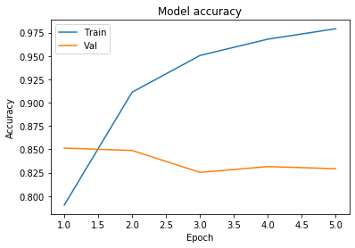

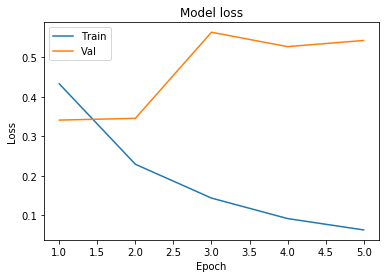
We can observe that the model is overfitting the training data. Overfitting happens when a model learns the detail and noise in the training data to the extent that it negatively impacts the performance of the model on new data. This means that the noise or random fluctuations in the training data is picked up and learned as concepts by the model. The problem is that these concepts do not apply to new data and negatively impact the models ability to generalize. Hence we are getting good accuracy on the training data but a lower accuracy on the test data. Dropout Layers can be an easy and effective way to prevent overfitting in your models. A dropout layer randomly drops some of the connections between layers.

Conclusion

In this tutorial you built an LSTM sentiment classifier on the IMDB dataset using Keras. After padding all reviews to 100 tokens and embedding them in 128-dimensional vectors, the single-layer LSTM reached 97.9% training accuracy after 5 epochs — but only 82.9% test accuracy, a clear sign of overfitting that the learning curves make visible.

Key takeaways:

• pad_sequences ensures all input sequences have the same fixed length, which is required for batch training; padding with zeros does not meaningfully affect learned representations for longer reviews.
• The trainable Embedding layer learns task-specific word vectors from scratch — for small datasets, pre-trained vectors (GloVe, Word2Vec) would reduce overfitting and boost test accuracy.
• Validation loss rising after epoch 2 while training loss keeps falling is the textbook overfitting signature; adding Dropout inside or after the LSTM is the first intervention to try.

Next steps:

• Add a Dropout(0.3) layer after the LSTM and compare test accuracy in a follow-up training run.
• Replace the LSTM Embedding with pre-trained GloVe vectors in Words Embedding using GloVe Vectors to improve generalization.
• Apply transformer-based fine-tuning for the same task in Sentiment Classification with DistilBERT.