Prediction of Google Stock Price using RNN
Stacked LSTM networks capture long-range temporal patterns across sequences, handling vanishing gradients through learned input, forget, and output gates. This tutorial builds a multi-layer LSTM in TensorFlow using a 60-day look-back window to predict Google stock opening prices.
Dataset
You can download the dataset from here
The data used in this notebook is from 19th August,2004 to 7th October,2019. The dataset consists of 7 columns which contain the date, opening price, highest price, lowest price, closing price, adjusted closing price and volume of share for each day.
Steps to build stock prediction model
- Data Preprocessing
- Building the RNN
- Making the prediction and visualization
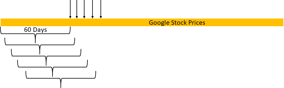
We will read the data for first 60 days and then predict for the 61st day. Then we will hop ahead bt one day and read the next chunk of data for next sixty days.
import numpy as np
import matplotlib.pyplot as plt
import pandas as pd
from sklearn.preprocessing import MinMaxScaler
read_csv is used to load the data into the dataframe. We can see the last 5 rows of the dataset using data.tail(). Similarly data.head() can be used to see the first 5 rows of the dataset. date_parser is used for converting a sequence of string columns to an array of datetime instances.
data = pd.read_csv('GOOG.csv', date_parser = True)
data.tail()| Date | Open | High | Low | Close | Adj Close | Volume | |
|---|---|---|---|---|---|---|---|
| 3804 | 2019-09-30 | 1220.969971 | 1226.000000 | 1212.300049 | 1219.000000 | 1219.000000 | 1404100 |
| 3805 | 2019-10-01 | 1219.000000 | 1231.229980 | 1203.579956 | 1205.099976 | 1205.099976 | 1273500 |
| 3806 | 2019-10-02 | 1196.979980 | 1196.979980 | 1171.290039 | 1176.630005 | 1176.630005 | 1615100 |
| 3807 | 2019-10-03 | 1180.000000 | 1189.060059 | 1162.430054 | 1187.829956 | 1187.829956 | 1621200 |
| 3808 | 2019-10-04 | 1191.890015 | 1211.439941 | 1189.170044 | 1209.000000 | 1209.000000 | 1021092 |
Here we splitting the data into training and testing dataset. We are going to take data from 2004 to 2018 as training data. Subsequently we are going to take the data of 2019 as testing data.
data_training = data[data['Date']='2019-01-01'].copy()We are dropping the columns Date and Adj Close from the training dataset
data_training = data_training.drop(['Date', 'Adj Close'], axis = 1)The values in the training data are not in the same range. For getting all the values in between the range 0 to 1 we are going to use MinMaxScalar().This improves the accuracy of prediction.
scaler = MinMaxScaler()
data_training = scaler.fit_transform(data_training)
data_trainingarray([[3.30294890e-04, 9.44785459e-04, 0.00000000e+00, 1.34908021e-04,
5.43577404e-01],
[7.42148227e-04, 2.98909923e-03, 1.88269054e-03, 3.39307537e-03,
2.77885613e-01],
[4.71386886e-03, 4.78092896e-03, 5.42828241e-03, 3.83867225e-03,
2.22150736e-01],
...,
[7.92197108e-01, 8.11970141e-01, 7.90196475e-01, 8.15799920e-01,
2.54672037e-02],
[8.18777193e-01, 8.21510648e-01, 8.20249255e-01, 8.10219301e-01,
1.70463908e-02],
[8.19874096e-01, 8.19172449e-01, 8.12332341e-01, 8.09012935e-01,
1.79975186e-02]])As mentioned above we are going to train the model on data of 60 days at a time. So the code mentioned below divides the data into chunks of 60 rows. data_training.shape[0] is equal to 3617 which corresponds to the length of data_traning. After dividing we are converting X_train and y_train into numpy arrays.
X_train = []
y_train = []

for i in range(60, data_training.shape[0]):
    X_train.append(data_training[i-60:i])
    y_train.append(data_training[i, 0])

X_train, y_train = np.array(X_train), np.array(y_train)
As we can see X_train now consists of 3557 chunks of data having 60 lists each and each list has 5 elements which correspond to the 5 attributes in the dataset.
X_train.shape(3557, 60, 5)Building LSTM
Here we are importing the necessary layers to build out neural network
from tensorflow.keras import Sequential
from tensorflow.keras.layers import Dense, LSTM, Dropout
The first layer is the LSTM layer with 60 units.
We will be using
reluactivation function.The rectified linear activation function or ReLU for short is a piecewise linear function that will output the input directly if it is positive, otherwise, it will output zero.
return_sequencewhen set toTruereturns the full sequence as the output.input_shapeis set to(X_train.shape[1],5)which is (60,5)Dropout layeris used to by randomly set the outgoing edges of hidden units to 0 at each update of the training phase.The value passed in dropout specifies the probability at which outputs of the layer are dropped out.
The last layer is the
Dense layeris the regular deeply connected neural network layer.As we are predicting a single value the
unitsin the last layer is set to 1.
regressor = Sequential()

regressor.add(LSTM(units = 60, activation = 'relu', return_sequences = True, input_shape = (X_train.shape[1], 5)))
regressor.add(Dropout(0.2))

regressor.add(LSTM(units = 60, activation = 'relu', return_sequences = True))
regressor.add(Dropout(0.2))

regressor.add(LSTM(units = 80, activation = 'relu', return_sequences = True))
regressor.add(Dropout(0.2))

regressor.add(LSTM(units = 120, activation = 'relu'))
regressor.add(Dropout(0.2))

regressor.add(Dense(units = 1))regressor.summary()Model: "sequential"
_________________________________________________________________
Layer (type) Output Shape Param #
=================================================================
lstm (LSTM) (None, 60, 60) 15840
_________________________________________________________________
dropout (Dropout) (None, 60, 60) 0
_________________________________________________________________
lstm_1 (LSTM) (None, 60, 60) 29040
_________________________________________________________________
dropout_1 (Dropout) (None, 60, 60) 0
_________________________________________________________________
lstm_2 (LSTM) (None, 60, 80) 45120
_________________________________________________________________
dropout_2 (Dropout) (None, 60, 80) 0
_________________________________________________________________
lstm_3 (LSTM) (None, 120) 96480
_________________________________________________________________
dropout_3 (Dropout) (None, 120) 0
_________________________________________________________________
dense (Dense) (None, 1) 121
=================================================================
Total params: 186,601
Trainable params: 186,601
Non-trainable params: 0
_________________________________________________________________Here we are compiling the model and fitting it to the training data. We will use 50 epochs to train the model. An epoch is an iteration over the entire data provided. batch_size is the number of samples per gradient update i.e. here the weights will be updates after 32 training examples.
regressor.compile(optimizer='adam', loss = 'mean_squared_error')
regressor.fit(X_train, y_train, epochs=50, batch_size=32)Train on 3557 samples
Epoch 45/50
3557/3557 [==============================] - 26s 7ms/sample - loss: 6.8088e-04
Epoch 46/50
3557/3557 [==============================] - 25s 7ms/sample - loss: 6.0968e-04
Epoch 47/50
3557/3557 [==============================] - 25s 7ms/sample - loss: 6.6604e-04
Epoch 48/50
3557/3557 [==============================] - 25s 7ms/sample - loss: 6.2150e-04
Epoch 49/50
3557/3557 [==============================] - 25s 7ms/sample - loss: 6.4292e-04
Epoch 50/50
3557/3557 [==============================] - 25s 7ms/sample - loss: 6.3066e-04Prepare test dataset
These are the first 5 entries in the test data set. To predict opening on any day we need the data of previous 60 days.
data_test.head()| Date | Open | High | Low | Close | Adj Close | Volume | |
|---|---|---|---|---|---|---|---|
| 3617 | 2019-01-02 | 1016.570007 | 1052.319946 | 1015.710022 | 1045.849976 | 1045.849976 | 1532600 |
| 3618 | 2019-01-03 | 1041.000000 | 1056.979980 | 1014.070007 | 1016.059998 | 1016.059998 | 1841100 |
| 3619 | 2019-01-04 | 1032.589966 | 1070.839966 | 1027.417969 | 1070.709961 | 1070.709961 | 2093900 |
| 3620 | 2019-01-07 | 1071.500000 | 1074.000000 | 1054.760010 | 1068.390015 | 1068.390015 | 1981900 |
| 3621 | 2019-01-08 | 1076.109985 | 1084.560059 | 1060.530029 | 1076.280029 | 1076.280029 | 1764900 |
past_60_days contains the data of the past 60 days required to predict the opening of the 1st day in the test data set.
past_60_days = data_training.tail(60)We are going to append data_test to past_60_days and ignore the index of data_test and drop Date and Adj Close.
df = past_60_days.append(data_test, ignore_index = True)
df = df.drop(['Date', 'Adj Close'], axis = 1)
df.head()| Open | High | Low | Close | Volume | |
|---|---|---|---|---|---|
| 0 | 1195.329956 | 1197.510010 | 1155.576050 | 1168.189941 | 2209500 |
| 1 | 1167.500000 | 1173.500000 | 1145.119995 | 1157.349976 | 1184300 |
| 2 | 1150.109985 | 1168.000000 | 1127.364014 | 1148.969971 | 1932400 |
| 3 | 1146.150024 | 1154.349976 | 1137.572021 | 1138.819946 | 1308700 |
| 4 | 1131.079956 | 1132.170044 | 1081.130005 | 1081.219971 | 2675700 |
Similar to the training data set we have to scale the test data so that all the values are in the range 0 to 1.
inputs = scaler.transform(df)
inputsarray([[0.93805611, 0.93755773, 0.92220906, 0.91781776, 0.0266752 ],
[0.91527437, 0.91792904, 0.91350452, 0.90892169, 0.01425359],
[0.90103881, 0.91343268, 0.89872289, 0.90204445, 0.02331778],
...,
[0.93940683, 0.93712442, 0.93529076, 0.9247443 , 0.01947328],
[0.92550693, 0.93064972, 0.92791493, 0.9339358 , 0.01954719],
[0.93524016, 0.94894575, 0.95017564, 0.95130949, 0.01227612]])We have to prepare the test data like the training data.
X_test = []
y_test = []

for i in range(60, inputs.shape[0]):
    X_test.append(inputs[i-60:i])
    y_test.append(inputs[i, 0])

X_test, y_test = np.array(X_test), np.array(y_test)
X_test.shape, y_test.shape((192, 60, 5), (192,))We are now going to predict the opening for X_test using predict()
y_pred = regressor.predict(X_test)As we had scaled all the values down, now we will have to get them back to the original scale. scaler.scale_ gives the scaling level
scaler.scale_array([8.18605127e-04, 8.17521128e-04, 8.32487534e-04, 8.20673293e-04,
1.21162775e-08])8.186 is the first value in the list which gives the scale of opening price. We will multiply y_pred and y_test with the inverse of this to get all the values to the original scale.
scale = 1/8.18605127e-04
scale1221.5901990069017y_pred = y_pred*scale
y_test = y_test*scaleVisualization
# Visualising the results
plt.figure(figsize=(14,5))
plt.plot(y_test, color = 'red', label = 'Real Google Stock Price')
plt.plot(y_pred, color = 'blue', label = 'Predicted Google Stock Price')
plt.title('Google Stock Price Prediction')
plt.xlabel('Time')
plt.ylabel('Google Stock Price')
plt.legend()
plt.show()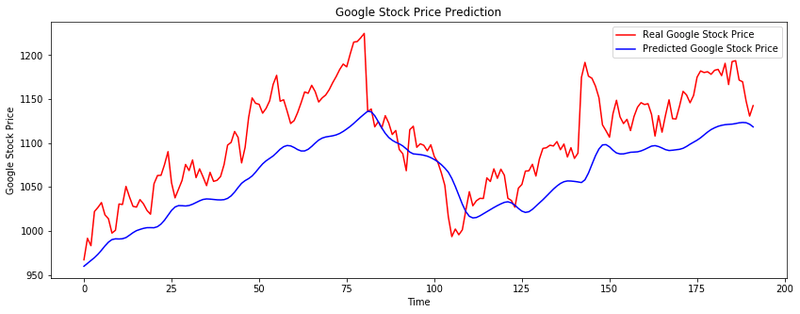
As we can see from the graph we have got a decent prediction of the opening price with a good accuracy.
Conclusion
In this tutorial you built a four-layer stacked LSTM in TensorFlow to predict Google's daily opening stock price using a 60-day look-back window on data from 2004 to 2018. The model successfully captured the general upward trend in 2019 prices, though sharp intra-month volatility remained difficult to predict precisely.
Key takeaways:
- A 60-day look-back window encodes enough historical context for the LSTM to detect medium-term trends; shorter windows lose context while longer ones require proportionally more training data.
- Stacking four LSTM layers with
Dropout(0.2)between them allows the model to learn increasingly abstract temporal representations while regularizing against overfitting. MinMaxScalermust be fit on training data only and then used to transform test data — leaking test statistics into the scaler creates an unrealistically optimistic evaluation.
Next steps:
- Compare the stacked LSTM approach to a single-layer LSTM in Airline Passenger Prediction using RNN-LSTM to see how architecture depth affects time-series accuracy.
- Apply multi-step forecasting in Multi-Step Time Series Prediction with LSTM to predict multiple days ahead rather than just one.
- Add technical indicators (SMA, RSI) as additional input features to give the LSTM richer context beyond raw OHLCV prices.