Household Power Consumption Prediction using RNN-LSTM
Power outage accidents will cause huge economic loss to the social economy. Therefore, it is very important to predict power consumption.
Given the rise of smart electricity meters and the wide adoption of electricity generation technology like solar panels, there is a wealth of electricity usage data available.

Problem Statement :
Given that power consumption data for the previous week, we have to predict the power consumption for the next week.
Watch Full Video:
Download dataset:
Download household_power_consumption.zip
Details:
UCI Household Electric Power Consumption dataset
Dataset Description:
The data was collected between December 2006 and November 2010 and observations of power consumption within the household were collected every minute.
It is a multivariate series comprised of seven variables
- global_active_power: The total active power consumed by the household (kilowatts).
- global_reactive_power: The total reactive power consumed by the household (kilowatts).
- voltage: Average voltage (volts).
- global_intensity: Average current intensity (amps).
- sub_metering_1: Active energy for kitchen (watt-hours of active energy).
- sub_metering_2: Active energy for laundry (watt-hours of active energy).
- sub_metering_3: Active energy for climate control systems (watt-hours of active energy).
This data represents a multivariate time series of power-related variables that in turn could be used to model and even forecast future electricity consumption
LSTM networks handle long-range temporal dependencies through gated memory cells, making them ideal for multi-step time-series forecasting. This tutorial builds an encoder-decoder LSTM in TensorFlow to forecast household power consumption seven days ahead using the UCI household electric power dataset.
Importing Libraries
import numpy as np
import pandas as pd
import matplotlib.pyplot as plt
from numpy import nan

from tensorflow.keras import Sequential
from tensorflow.keras.layers import LSTM, Dense

from sklearn.metrics import mean_squared_error
from sklearn.preprocessing import MinMaxScaler
python
#Reading the dataset

data = pd.read_csv('household_power_consumption.txt', sep = ';',
                  parse_dates = True,
low_memory = False)#printing top rows
data.head()| Date | Time | Global_active_power | Global_reactive_power | Voltage | Global_intensity | Sub_metering_1 | Sub_metering_2 | Sub_metering_3 | |
|---|---|---|---|---|---|---|---|---|---|
| 0 | 16/12/2006 | 17:24:00 | 4.216 | 0.418 | 234.840 | 18.400 | 0.000 | 1.000 | 17.0 |
| 1 | 16/12/2006 | 17:25:00 | 5.360 | 0.436 | 233.630 | 23.000 | 0.000 | 1.000 | 16.0 |
| 2 | 16/12/2006 | 17:26:00 | 5.374 | 0.498 | 233.290 | 23.000 | 0.000 | 2.000 | 17.0 |
| 3 | 16/12/2006 | 17:27:00 | 5.388 | 0.502 | 233.740 | 23.000 | 0.000 | 1.000 | 17.0 |
| 4 | 16/12/2006 | 17:28:00 | 3.666 | 0.528 | 235.680 | 15.800 | 0.000 | 1.000 | 17.0 |
#concatenating the date and time columns to 'date_time' columns

data['date_time'] = data['Date'].str.cat(data['Time'], sep= ' ')
data.drop(['Date', 'Time'], inplace= True, axis = 1)
data.head()| Global_active_power | Global_reactive_power | Voltage | Global_intensity | Sub_metering_1 | Sub_metering_2 | Sub_metering_3 | date_time | |
|---|---|---|---|---|---|---|---|---|
| 0 | 4.216 | 0.418 | 234.840 | 18.400 | 0.000 | 1.000 | 17.0 | 16/12/2006 17:24:00 |
| 1 | 5.360 | 0.436 | 233.630 | 23.000 | 0.000 | 1.000 | 16.0 | 16/12/2006 17:25:00 |
| 2 | 5.374 | 0.498 | 233.290 | 23.000 | 0.000 | 2.000 | 17.0 | 16/12/2006 17:26:00 |
| 3 | 5.388 | 0.502 | 233.740 | 23.000 | 0.000 | 1.000 | 17.0 | 16/12/2006 17:27:00 |
| 4 | 3.666 | 0.528 | 235.680 | 15.800 | 0.000 | 1.000 | 17.0 | 16/12/2006 17:28:00 |
data.set_index(['date_time'], inplace=True)
data.head()| date_time | Global_active_power | Global_reactive_power | Voltage | Global_intensity | Sub_metering_1 | Sub_metering_2 | Sub_metering_3 |
|---|---|---|---|---|---|---|---|
| 16/12/2006 17:24:00 | 4.216 | 0.418 | 234.840 | 18.400 | 0.000 | 1.000 | 17.0 |
| 16/12/2006 17:25:00 | 5.360 | 0.436 | 233.630 | 23.000 | 0.000 | 1.000 | 16.0 |
| 16/12/2006 17:26:00 | 5.374 | 0.498 | 233.290 | 23.000 | 0.000 | 2.000 | 17.0 |
| 16/12/2006 17:27:00 | 5.388 | 0.502 | 233.740 | 23.000 | 0.000 | 1.000 | 17.0 |
| 16/12/2006 17:28:00 | 3.666 | 0.528 | 235.680 | 15.800 | 0.000 | 1.000 | 17.0 |
Next, we can mark all missing values indicated with a ‘?‘ character with a NaN value, which is a float.
#replacing each '?'characters with NaN value

data.replace('?', nan, inplace=True)#This will allow us to work with the data as one array of floating point values rather than mixed types (less efficient.)
data = data.astype('float')#information of the dataset
data.info()Index: 2075259 entries, 16/12/2006 17:24:00 to 26/11/2010 21:02:00
Data columns (total 7 columns):
Global_active_power float64
Global_reactive_power float64
Voltage float64
Global_intensity float64
Sub_metering_1 float64
Sub_metering_2 float64
Sub_metering_3 float64
dtypes: float64(7)
memory usage: 126.7+ MB#checking the null values
np.isnan(data).sum()Global_active_power 25979
Global_reactive_power 25979
Voltage 25979
Global_intensity 25979
Sub_metering_1 25979
Sub_metering_2 25979
Sub_metering_3 25979
dtype: int64We also need to fill in the missing values now that they have been marked.
A very simple approach would be to copy the observation from the same time the day before. We can implement this in a function named fill_missing() that will take the NumPy array of the data and copy values from exactly 24 hours ago.
def fill_missing(data):
    one_day = 24*60
    for row in range(data.shape[0]):
        for col in range(data.shape[1]):
            if np.isnan(data[row, col]):
data[row, col] = data[row-one_day, col]fill_missing(data.values)#checking the nan values
np.isnan(data).sum()Global_active_power 0
Global_reactive_power 0
Voltage 0
Global_intensity 0
Sub_metering_1 0
Sub_metering_2 0
Sub_metering_3 0
dtype: int64data.info()Index: 2075259 entries, 16/12/2006 17:24:00 to 26/11/2010 21:02:00
Data columns (total 7 columns):
Global_active_power float64
Global_reactive_power float64
Voltage float64
Global_intensity float64
Sub_metering_1 float64
Sub_metering_2 float64
Sub_metering_3 float64
dtypes: float64(7)
memory usage: 126.7+ MB
#printing the shape of the data
data.shape
(2075259, 7)Here, we can observe that we have 2075259 datapoints and 7 features
data.head()| date_time | Global_active_power | Global_reactive_power | Voltage | Global_intensity | Sub_metering_1 | Sub_metering_2 | Sub_metering_3 |
|---|---|---|---|---|---|---|---|
| 16/12/2006 17:24:00 | 4.216 | 0.418 | 234.84 | 18.4 | 0.0 | 1.0 | 17.0 |
| 16/12/2006 17:25:00 | 5.360 | 0.436 | 233.63 | 23.0 | 0.0 | 1.0 | 16.0 |
| 16/12/2006 17:26:00 | 5.374 | 0.498 | 233.29 | 23.0 | 0.0 | 2.0 | 17.0 |
| 16/12/2006 17:27:00 | 5.388 | 0.502 | 233.74 | 23.0 | 0.0 | 1.0 | 17.0 |
| 16/12/2006 17:28:00 | 3.666 | 0.528 | 235.68 | 15.8 | 0.0 | 1.0 | 17.0 |
Prepare power consumption for each day
We can now save the cleaned-up version of the dataset to a new file; in this case we will just change the file extension to .csv and save the dataset as ‘cleaned_data.csv‘.
#conversion of dataframe to .csv

data.to_csv('cleaned_data.csv')#reading the dataset
dataset = pd.read_csv('cleaned_data.csv', parse_dates = True, index_col = 'date_time', low_memory = False)#printing the top rows
dataset.head()| date_time | Global_active_power | Global_reactive_power | Voltage | Global_intensity | Sub_metering_1 | Sub_metering_2 | Sub_metering_3 |
|---|---|---|---|---|---|---|---|
| 2006-12-16 17:24:00 | 4.216 | 0.418 | 234.84 | 18.4 | 0.0 | 1.0 | 17.0 |
| 2006-12-16 17:25:00 | 5.360 | 0.436 | 233.63 | 23.0 | 0.0 | 1.0 | 16.0 |
| 2006-12-16 17:26:00 | 5.374 | 0.498 | 233.29 | 23.0 | 0.0 | 2.0 | 17.0 |
| 2006-12-16 17:27:00 | 5.388 | 0.502 | 233.74 | 23.0 | 0.0 | 1.0 | 17.0 |
| 2006-12-16 17:28:00 | 3.666 | 0.528 | 235.68 | 15.8 | 0.0 | 1.0 | 17.0 |
#printing the bottom rows

dataset.tail()| date_time | Global_active_power | Global_reactive_power | Voltage | Global_intensity | Sub_metering_1 | Sub_metering_2 | Sub_metering_3 |
|---|---|---|---|---|---|---|---|
| 2010-11-26 20:58:00 | 0.946 | 0.0 | 240.43 | 4.0 | 0.0 | 0.0 | 0.0 |
| 2010-11-26 20:59:00 | 0.944 | 0.0 | 240.00 | 4.0 | 0.0 | 0.0 | 0.0 |
| 2010-11-26 21:00:00 | 0.938 | 0.0 | 239.82 | 3.8 | 0.0 | 0.0 | 0.0 |
| 2010-11-26 21:01:00 | 0.934 | 0.0 | 239.70 | 3.8 | 0.0 | 0.0 | 0.0 |
| 2010-11-26 21:02:00 | 0.932 | 0.0 | 239.55 | 3.8 | 0.0 | 0.0 | 0.0 |
Exploratory Data Analysis
#Downsampling the data into dáy-wise bins and sum the values of the timestamps falling into a bin.

data = dataset.resample('D').sum()#data after sampling it into daywise manner
data.head()| date_time | Global_active_power | Global_reactive_power | Voltage | Global_intensity | Sub_metering_1 | Sub_metering_2 | Sub_metering_3 |
|---|---|---|---|---|---|---|---|
| 2006-12-16 | 1209.176 | 34.922 | 93552.53 | 5180.8 | 0.0 | 546.0 | 4926.0 |
| 2006-12-17 | 3390.460 | 226.006 | 345725.32 | 14398.6 | 2033.0 | 4187.0 | 13341.0 |
| 2006-12-18 | 2203.826 | 161.792 | 347373.64 | 9247.2 | 1063.0 | 2621.0 | 14018.0 |
| 2006-12-19 | 1666.194 | 150.942 | 348479.01 | 7094.0 | 839.0 | 7602.0 | 6197.0 |
| 2006-12-20 | 2225.748 | 160.998 | 348923.61 | 9313.0 | 0.0 | 2648.0 | 14063.0 |
Plotting the all features in various time stamps
fig, ax = plt.subplots(figsize=(18,18))

for i in range(len(data.columns)):
    plt.subplot(len(data.columns), 1, i+1)
    name = data.columns[i]
    plt.plot(data[name])
    plt.title(name, y=0, loc = 'right')
    plt.yticks([])
plt.show()
fig.tight_layout()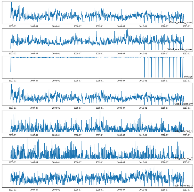
Exploring Active power consumption for each year
#we have considered 5 years here

years = ['2007', '2008', '2009', '2010']
Year wise plotting of feature Global_active_power
fig, ax = plt.subplots(figsize=(18,18))

for i in range(len(years)):
    plt.subplot(len(years), 1, i+1)
    year = years[i]
    active_power_data = data[str(year)]
    plt.plot(active_power_data['Global_active_power'])
    plt.title(str(year), y = 0, loc = 'left')
plt.show()
fig.tight_layout()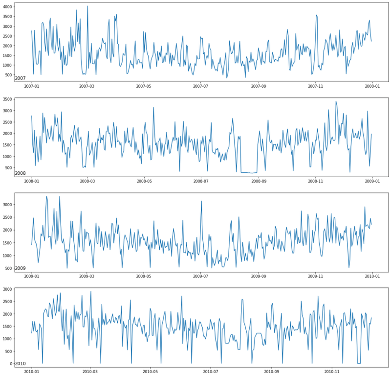
#for year 2006

data['2006']| date_time | Global_active_power | Global_reactive_power | Voltage | Global_intensity | Sub_metering_1 | Sub_metering_2 | Sub_metering_3 |
|---|---|---|---|---|---|---|---|
| 2006-12-16 | 1209.176 | 34.922 | 93552.53 | 5180.8 | 0.0 | 546.0 | 4926.0 |
| 2006-12-17 | 3390.460 | 226.006 | 345725.32 | 14398.6 | 2033.0 | 4187.0 | 13341.0 |
| 2006-12-18 | 2203.826 | 161.792 | 347373.64 | 9247.2 | 1063.0 | 2621.0 | 14018.0 |
| 2006-12-19 | 1666.194 | 150.942 | 348479.01 | 7094.0 | 839.0 | 7602.0 | 6197.0 |
| 2006-12-20 | 2225.748 | 160.998 | 348923.61 | 9313.0 | 0.0 | 2648.0 | 14063.0 |
| 2006-12-21 | 1723.288 | 144.434 | 347096.41 | 7266.4 | 1765.0 | 2692.0 | 10456.0 |
| 2006-12-22 | 2341.338 | 186.906 | 347305.75 | 9897.0 | 3151.0 | 350.0 | 11131.0 |
| 2006-12-23 | 4773.386 | 221.470 | 345795.95 | 20200.4 | 2669.0 | 425.0 | 14726.0 |
| 2006-12-24 | 2550.012 | 149.900 | 348029.91 | 11002.2 | 1703.0 | 5082.0 | 6891.0 |
| 2006-12-25 | 2743.120 | 240.280 | 350495.90 | 11450.2 | 6620.0 | 1962.0 | 5795.0 |
| 2006-12-26 | 3934.110 | 165.102 | 347940.63 | 16341.0 | 1086.0 | 2533.0 | 14979.0 |
| 2006-12-27 | 1528.760 | 178.902 | 351025.00 | 6505.2 | 0.0 | 314.0 | 6976.0 |
| 2006-12-28 | 2072.638 | 208.876 | 350306.40 | 8764.2 | 2207.0 | 4419.0 | 9176.0 |
| 2006-12-29 | 3174.392 | 196.394 | 346854.68 | 13350.8 | 1252.0 | 5162.0 | 11329.0 |
| 2006-12-30 | 2796.108 | 312.142 | 346377.15 | 11952.6 | 3072.0 | 7893.0 | 12516.0 |
| 2006-12-31 | 3494.196 | 150.852 | 345451.07 | 14687.4 | 0.0 | 347.0 | 6502.0 |
Power consumption distribution with histogram
Year wise histogram plot of feature Global_active_power
fig, ax = plt.subplots(figsize=(18,18))

for i in range(len(years)):
    plt.subplot(len(years), 1, i+1)
    year = years[i]
    active_power_data = data[str(year)]
    active_power_data['Global_active_power'].hist(bins = 200)
    plt.title(str(year), y = 0, loc = 'left')
plt.show()
fig.tight_layout()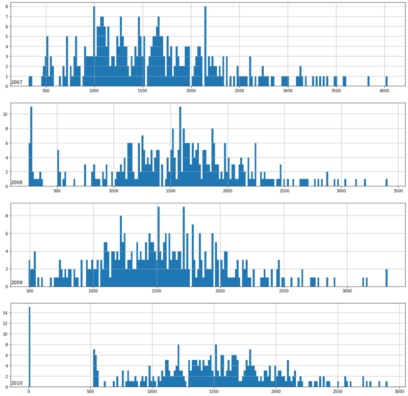
Histogram plot for All Features
fig, ax = plt.subplots(figsize=(18,18))

for i in range(len(data.columns)):
    plt.subplot(len(data.columns), 1, i+1)
    name = data.columns[i]
    data[name].hist(bins=200)
    plt.title(name, y=0, loc = 'right')
    plt.yticks([])
plt.show()
fig.tight_layout()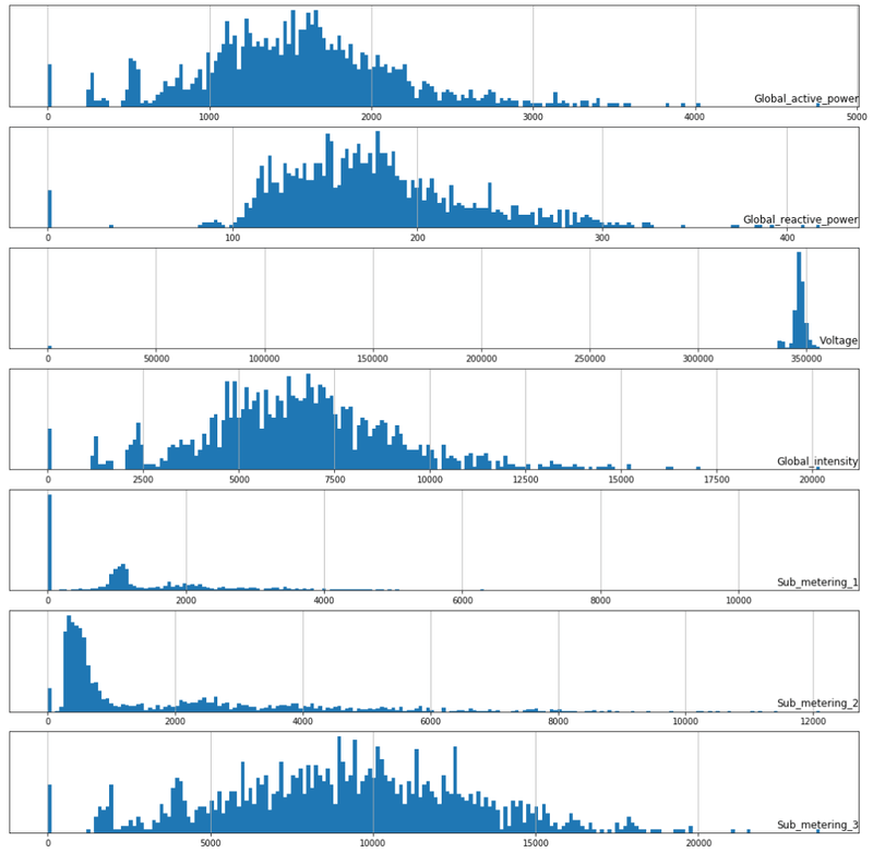
Plot power consumption hist for each month of 2007
months = [i for i in range(1,13)]

fig, ax = plt.subplots(figsize=(18,18))

for i in range(len(months)):
    ax = plt.subplot(len(months), 1, i+1)
    month = '2007-' + str(months[i])
    active_power_data = dataset[month]
    active_power_data['Global_active_power'].hist(bins = 100)
    ax.set_xlim(0,5)
    plt.title(month, y = 0, loc = 'right')
plt.show()
fig.tight_layout()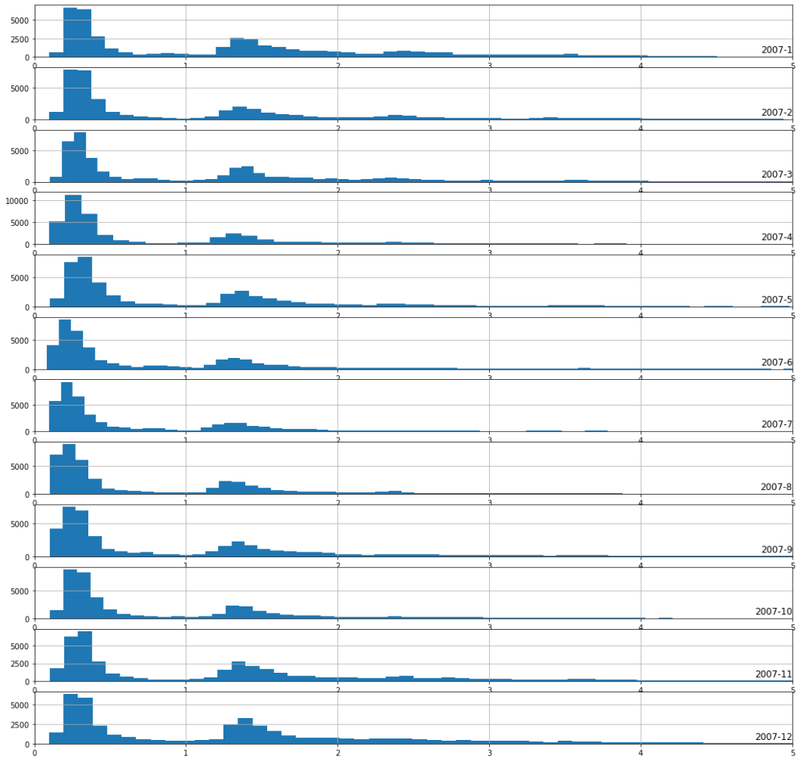
Observation :
From the above diagram we can say that power consumption in the month of Nov, Dec, Jan, Feb, Mar is more as there is a long tail as compare to other months.
It also shows that the during the winter seasons, the heating systems are used and not in summer.
The above graph is highly concentrated on 0.3W and 1.3W.
Active Power Uses Prediction
What can we predict
- Forecast hourly consumption for the next day.
- Forecast daily consumption for the next week.
- Forecast daily consumption for the next month.
- Forecast monthly consumption for the next year.
Modeling Methods
There are many modeling methods and few of those are as follows
- Naive Methods -> Naive methods would include methods that make very simple, but often very effective assumptions.
- Classical Linear Methods -> Classical linear methods include techniques are very effective for univariate time series forecasting
- Machine Learning Methods -> Machine learning methods require that the problem be framed as a supervised learning problem.K-nearest neighbors.
- SVM
- Decision trees
- Random forest
- Gradient boosting machines
- CNN
- LSTM
- CNN - LSTM
Problem Framing:
Given recent power consumption, what is the expected power consumption for the week ahead?
This requires that a predictive model forecast the total active power for each day over the next seven days
A model of this type could be helpful within the household in planning expenditures. It could also be helpful on the supply side for planning electricity demand for a specific household.
Input -> Predict
[Week1] -> Week2
[Week2] -> Week3
[Week3] -> Week4
#top rows

data.head()| date_time | Global_active_power | Global_reactive_power | Voltage | Global_intensity | Sub_metering_1 | Sub_metering_2 | Sub_metering_3 |
|---|---|---|---|---|---|---|---|
| 2006-12-16 | 1209.176 | 34.922 | 93552.53 | 5180.8 | 0.0 | 546.0 | 4926.0 |
| 2006-12-17 | 3390.460 | 226.006 | 345725.32 | 14398.6 | 2033.0 | 4187.0 | 13341.0 |
| 2006-12-18 | 2203.826 | 161.792 | 347373.64 | 9247.2 | 1063.0 | 2621.0 | 14018.0 |
| 2006-12-19 | 1666.194 | 150.942 | 348479.01 | 7094.0 | 839.0 | 7602.0 | 6197.0 |
| 2006-12-20 | 2225.748 | 160.998 | 348923.61 | 9313.0 | 0.0 | 2648.0 | 14063.0 |
#printing last rows

data.tail()| date_time | Global_active_power | Global_reactive_power | Voltage | Global_intensity | Sub_metering_1 | Sub_metering_2 | Sub_metering_3 |
|---|---|---|---|---|---|---|---|
| 2010-12-07 | 1109.574 | 285.912 | 345914.85 | 4892.0 | 1724.0 | 646.0 | 6444.0 |
| 2010-12-08 | 529.698 | 169.098 | 346744.70 | 2338.2 | 0.0 | 514.0 | 3982.0 |
| 2010-12-09 | 1612.092 | 201.358 | 347932.40 | 6848.2 | 1805.0 | 2080.0 | 8891.0 |
| 2010-12-10 | 1579.692 | 170.268 | 345975.37 | 6741.2 | 1104.0 | 780.0 | 9812.0 |
| 2010-12-11 | 1836.822 | 151.144 | 343926.57 | 7826.2 | 2054.0 | 489.0 | 10308.0 |
#here are splitting the dataset
#dataset upto end of 2009 is in train dataset and remaining we keeping it in test dataset

data_train = data.loc[:'2009-12-31', :]['Global_active_power']
data_train.head()date_time
2006-12-16 1209.176
2006-12-17 3390.460
2006-12-18 2203.826
2006-12-19 1666.194
2006-12-20 2225.748
Freq: D, Name: Global_active_power, dtype: float64data_test = data['2010']['Global_active_power']
data_test.head()date_time
2010-01-01 1224.252
2010-01-02 1693.778
2010-01-03 1298.728
2010-01-04 1687.440
2010-01-05 1320.158
Freq: D, Name: Global_active_power, dtype: float64data_train.shape(1112,)data_test.shape(345,)Observation :
- We have 1112 datapoints in train dataset and 345 datapoints in test dataset
Prepare training data
#training data

data_train.head(14)date_time
2006-12-16 1209.176
2006-12-17 3390.460
2006-12-18 2203.826
2006-12-19 1666.194
2006-12-20 2225.748
2006-12-21 1723.288
2006-12-22 2341.338
2006-12-23 4773.386
2006-12-24 2550.012
2006-12-25 2743.120
2006-12-26 3934.110
2006-12-27 1528.760
2006-12-28 2072.638
2006-12-29 3174.392
Freq: D, Name: Global_active_power, dtype: float64#converting the data into numpy array
data_train = np.array(data_train)#we are splitting the data weekly wise(7days)
X_train, y_train = [], []
for i in range(7, len(data_train)-7):
X_train.append(data_train[i-7:i])
y_train.append(data_train[i:i+7])#converting list to numpy array
X_train, y_train = np.array(X_train), np.array(y_train)#shape of train and test dataset
X_train.shape, y_train.shape
((1098, 7), (1098, 7))#printing the ytrain value
pd.DataFrame(y_train).head()| 0 | 1 | 2 | 3 | 4 | 5 | 6 | |
|---|---|---|---|---|---|---|---|
| 0 | 4773.386 | 2550.012 | 2743.120 | 3934.110 | 1528.760 | 2072.638 | 3174.392 |
| 1 | 2550.012 | 2743.120 | 3934.110 | 1528.760 | 2072.638 | 3174.392 | 2796.108 |
| 2 | 2743.120 | 3934.110 | 1528.760 | 2072.638 | 3174.392 | 2796.108 | 3494.196 |
| 3 | 3934.110 | 1528.760 | 2072.638 | 3174.392 | 2796.108 | 3494.196 | 2749.004 |
| 4 | 1528.760 | 2072.638 | 3174.392 | 2796.108 | 3494.196 | 2749.004 | 1824.760 |
#Normalising the dataset between 0 and 1

x_scaler = MinMaxScaler()
X_train = x_scaler.fit_transform(X_train)#Normalising the dataset
y_scaler = MinMaxScaler()
y_train = y_scaler.fit_transform(y_train)pd.DataFrame(X_train).head()| 0 | 1 | 2 | 3 | 4 | 5 | 6 | |
|---|---|---|---|---|---|---|---|
| 0 | 0.211996 | 0.694252 | 0.431901 | 0.313037 | 0.436748 | 0.325660 | 0.462304 |
| 1 | 0.694252 | 0.431901 | 0.313037 | 0.436748 | 0.325660 | 0.462304 | 1.000000 |
| 2 | 0.431901 | 0.313037 | 0.436748 | 0.325660 | 0.462304 | 1.000000 | 0.508439 |
| 3 | 0.313037 | 0.436748 | 0.325660 | 0.462304 | 1.000000 | 0.508439 | 0.551133 |
| 4 | 0.436748 | 0.325660 | 0.462304 | 1.000000 | 0.508439 | 0.551133 | 0.814446 |
#converting to 3 dimension

X_train = X_train.reshape(1098, 7, 1)X_train.shape(1098, 7, 1)Build LSTM Model
#building sequential model using Keras

reg = Sequential()
reg.add(LSTM(units = 200, activation = 'relu', input_shape=(7,1)))
reg.add(Dense(7))#here we have considered loss as mean square error and optimizer as adam
reg.compile(loss='mse', optimizer='adam')#training the model
reg.fit(X_train, y_train, epochs = 100)Train on 1098 samples
Epoch 1/100
1098/1098 [==============================] - 2s 2ms/sample - loss: 0.0626
Epoch 2/100
1098/1098 [==============================] - 0s 296us/sample -
.
.
.
.
.
Epoch 99/100
1098/1098 [==============================] - 0s 270us/sample - loss: 0.0228
Epoch 100/100
1098/1098 [==============================] - 0s 269us/sample - loss: 0.0228Observation:
- We have done with training and loss which we have got is 0.0232
Prepare test dataset and test LSTM model
#testing dataset

data_test = np.array(data_test)#here we are splitting the data weekly wise(7days)
X_test, y_test = [], []
for i in range(7, len(data_test)-7):
X_test.append(data_test[i-7:i])
y_test.append(data_test[i:i+7])X_test, y_test = np.array(X_test), np.array(y_test)X_test = x_scaler.transform(X_test)
y_test = y_scaler.transform(y_test)#converting to 3 dimension
X_test = X_test.reshape(331,7,1)X_test.shape(331, 7, 1)y_pred = reg.predict(X_test)#bringing y_pred values to their original forms by using inverse transform
y_pred = y_scaler.inverse_transform(y_pred)y_predarray([[1508.9413 , 1476.1537 , 1487.5676 , ..., 1484.8464 , 1459.3864 ,
1551.5675 ],
[1158.2788 , 1287.0326 , 1346.428 , ..., 1430.5685 , 1420.6346 ,
1472.5759 ],
[1571.7665 , 1507.0337 , 1516.5574 , ..., 1432.5813 , 1393.9161 ,
1504.1714 ],
...,
[ 952.85785, 852.4236 , 933.62585, ..., 800.12006, 831.2844 ,
1005.20844],
[1579.4896 , 1353.6078 , 1278.9501 , ..., 981.4198 , 967.6466 ,
1146.7898 ],
[1629.0509 , 1392.7751 , 1288.7218 , ..., 1052.977 , 1070.8586 ,
1243.1346 ]], dtype=float32)y_true = y_scaler.inverse_transform(y_test)y_truearray([[ 555.664, 1593.318, 1504.82 , ..., 0. , 1995.796, 2116.224],
[1593.318, 1504.82 , 1383.18 , ..., 1995.796, 2116.224, 2196.76 ],
[1504.82 , 1383.18 , 0. , ..., 2116.224, 2196.76 , 2150.112],
...,
[1892.998, 1645.424, 1439.426, ..., 1973.382, 1109.574, 529.698],
[1645.424, 1439.426, 2035.418, ..., 1109.574, 529.698, 1612.092],
[1439.426, 2035.418, 1973.382, ..., 529.698, 1612.092, 1579.692]])Evaluate the model
Here, we using metric as mean square error since it is a regression problem
def evaluate_model(y_true, y_predicted):
    scores = []

    #calculate scores for each day
    for i in range(y_true.shape[1]):
        mse = mean_squared_error(y_true[:, i], y_predicted[:, i])
        rmse = np.sqrt(mse)
        scores.append(rmse)

    #calculate score for whole prediction
    total_score = 0
    for row in range(y_true.shape[0]):
        for col in range(y_predicted.shape[1]):
            total_score = total_score + (y_true[row, col] - y_predicted[row, col])**2
    total_score = np.sqrt(total_score/(y_true.shape[0]*y_predicted.shape[1]))

return total_score, scoresevaluate_model(y_true, y_pred)(579.2827596682928, [598.0411885086157, 592.5770673397814, 576.1153945912635, 563.9396525162248, 576.5479538079353, 570.7699415990154, 576.2430188855649])#standard deviation
np.std(y_true[0])710.0253857243853Conclusion
In this tutorial you built an encoder LSTM that forecasts household power consumption seven days ahead using the UCI dataset resampled to daily resolution. The model achieved an overall RMSE of 579 watts against a target standard deviation of 710 watts, confirming it outperforms a naive baseline. Per-day RMSE ranged from 564 W (day 4) to 598 W (day 1), showing the model is most uncertain about next-day predictions.
Key takeaways:
- Resampling minute-level sensor data to daily sums with
.resample("D").sum()reduces noise and aligns the input granularity with the forecasting horizon, making patterns easier to learn. - Framing multi-step forecasting as a direct multi-output regression (predicting all 7 days at once) with a single
Dense(7)output is simpler and often competitive with autoregressive approaches. - Fit
MinMaxScaleron training data only and apply.transform()on test data to prevent data leakage — always inverse-transform predictions before computing RMSE for interpretable error units. - RMSE < standard deviation of the target confirms the model adds value; when they are equal, the model is no better than always predicting the mean.
Next steps:
- Replace the simple LSTM with an encoder-decoder architecture (Repeat Vector + second LSTM decoder) to better model the sequence-to-sequence nature of the 7-day output.
- Compare against Google Stock Price Prediction using RNN-LSTM to see single-step vs. multi-step forecasting trade-offs.
- Predict all 7 sensor variables simultaneously (not just
Global_active_power) to leverage the multivariate structure of the dataset.