ModernBERT is an encoder that Answer.AI and LightOn released in December 2024, under the Apache 2.0 license. The base model has 149M parameters, reads up to 8,192 tokens at once and was trained on 2 trillion tokens of English text and code. It does not write text. It reads text and gives back one vector per token, the kind of vector that search, classification and tagging systems are built on.
In this blog, we will learn how ModernBERT-base works by running real code on it. We will follow short sentences from text to tokens, through 22 encoder layers, to one vector per token and then one vector per text. On the way, we will see what each part does, where the weights sit and how an encoder learns by filling in blanks.
What Is ModernBERT-base?
ModernBERT is built on the Transformer, the design from the 2017 paper "Attention Is All You Need" by Vaswani et al. So before we open ModernBERT, let's look at that original model as below.
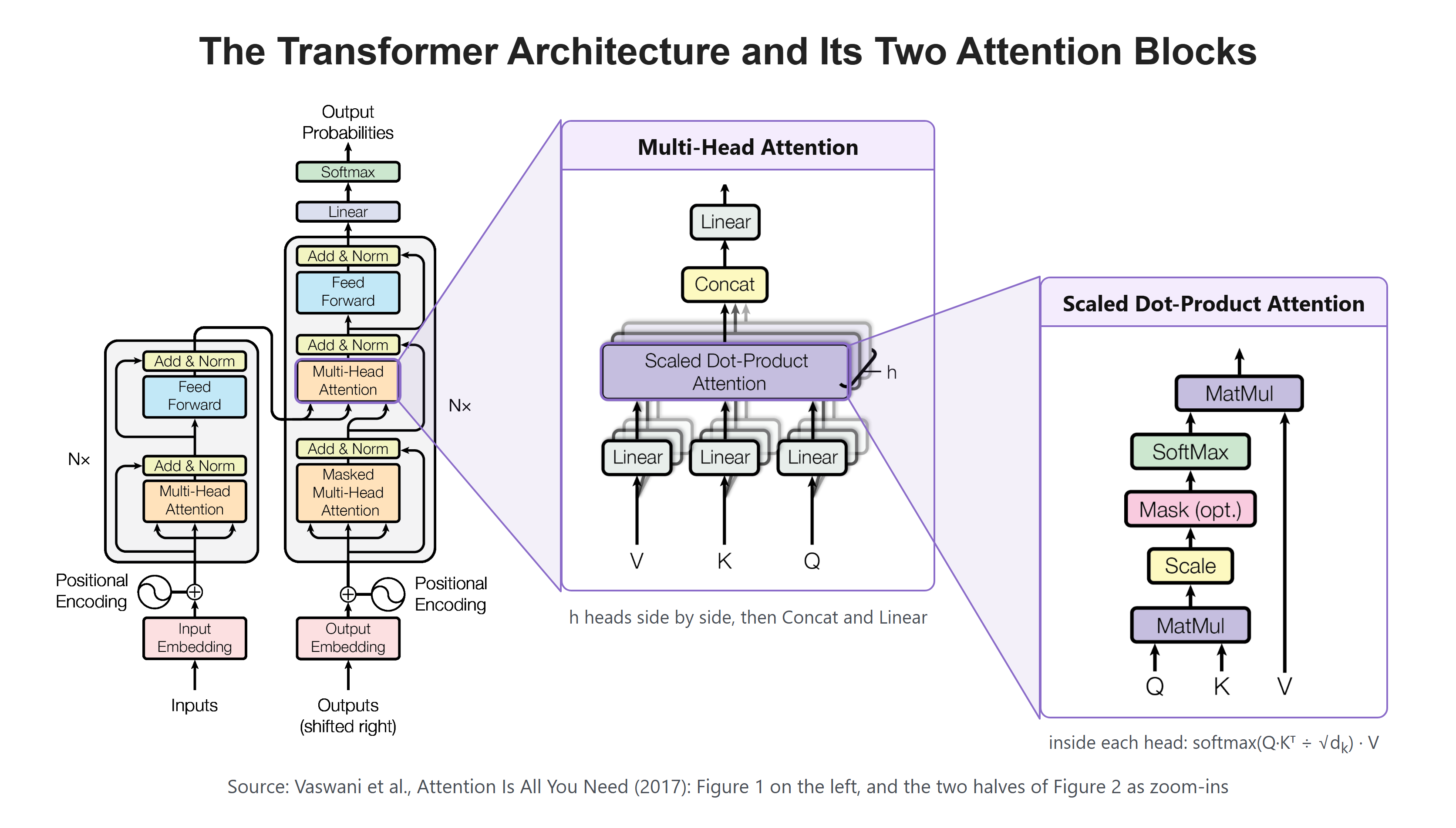
Here, we can see two towers. The left tower is the encoder. Its Multi-Head Attention has no mask, so every token can look at every other token, the ones before it and the ones after it. The right tower is the decoder, which writes text one token at a time. ModernBERT keeps only the encoder tower. The "Nx" next to the tower means the layer is stacked N times, and in ModernBERT-base N is 22. The two zoom-ins on the right show Multi-Head Attention and the Scaled Dot-Product Attention inside each head, and ModernBERT still runs that same attention in every layer.
The name comes from BERT, the encoder Google released in 2018. BERT learned by guessing hidden words, and ModernBERT learns the same way. But BERT could read only 512 tokens, and many of its parts date from 2018. ModernBERT keeps the job and swaps the parts for newer ones. Its training also hides 30% of the tokens instead of BERT's 15%, and it drops BERT's second task, next-sentence prediction.
Let me tabulate the main settings for your better understanding.
| Setting | Value |
|---|---|
| Parameters | 149,014,272 (149M) |
| Encoder layers | 22 (8 global, 14 local) |
| Hidden size (numbers per token) | 768 |
| Attention heads | 12, each 64 numbers wide |
| MLP size | 1,152 (Wi makes 2 × 1,152) |
| Vocabulary | 50,368 |
| Context length | 8,192 tokens |
| Local attention window | 128 tokens, 64 on each side |
| Positions | RoPE, base 160,000 (global) and 10,000 (local) |
| Norm | LayerNorm without bias, eps 1e-5 |
| MLP activation | GELU, inside a GeGLU MLP |
| Biases | none, except the masked-LM decoder |
| Stored weights | float32 |
The picture below shows the whole model at once. On the left is the full stack: a token embedding, 22 encoder layers and a final LayerNorm. The middle panel zooms into one encoder layer, and the right panels zoom into its MLP and its attention.
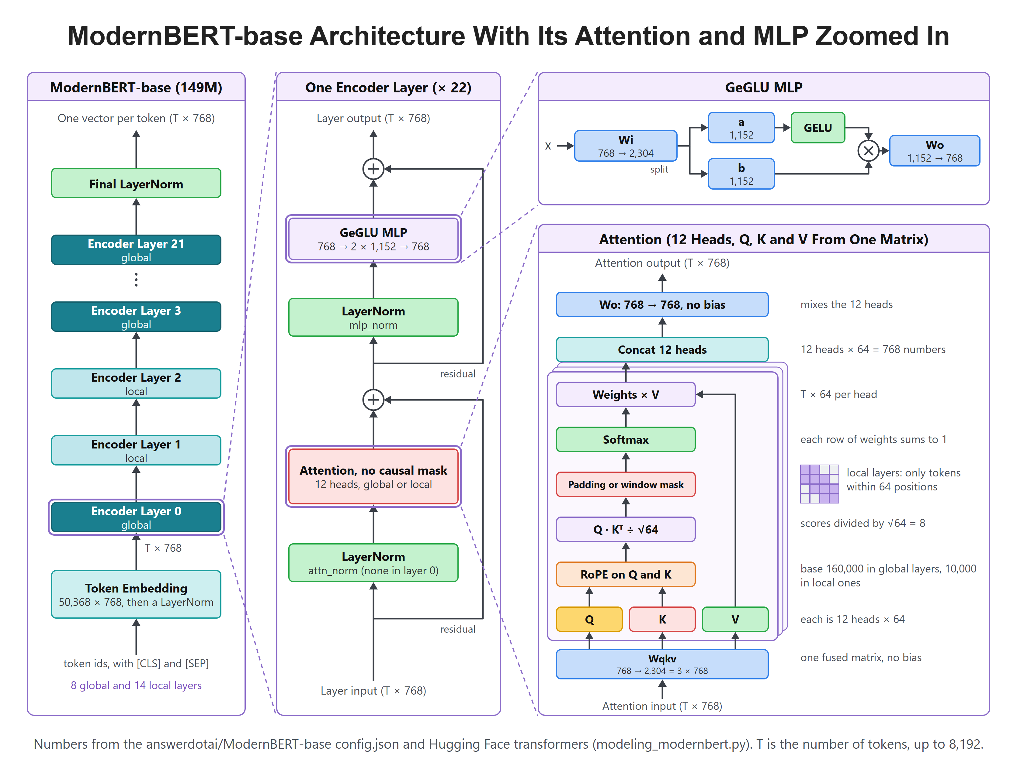
Here, we can see three things that stand out. There is no causal mask, so attention reads in both directions. The layers come in two kinds: every third layer is global and sees the whole text, and the rest are local and see only nearby tokens. And Q, K and V all come out of one matrix, Wqkv. We will open every one of these boxes with code.
ModernBERT keeps the plan of the original Transformer's encoder: a stack of identical layers, each with self-attention and an MLP, joined by residual connections. But four parts inside the layer are newer than the 2017 paper: LayerNorm without bias placed before each block, RoPE, local and global attention, and GeGLU. The ModernBERT paper also strips padding tokens out before the layers run and uses Flash Attention, which make it fast. We will meet each part below.
Our Test Setup
We run every example on one NVIDIA GeForce RTX 5090 (32 GB) with PyTorch 2.11.0 and Hugging Face transformers 5.17.0. The model loads in its stored format, float32. We never train anything, so gradients are switched off for the whole blog.
Every number in this blog, and in every figure, comes from the code below. The examples follow the course notebook: the same sentences, the same random seeds and the same order of steps.
Let's see the code as below. It loads the tokenizer and the model, then prints the model:
import torch
import matplotlib.pyplot as plt
from transformers import AutoTokenizer, AutoModel, AutoModelForSequenceClassification, pipeline, logging

torch.set_grad_enabled(False)
logging.set_verbosity_error()

MODEL = "answerdotai/ModernBERT-base"

tok = AutoTokenizer.from_pretrained(MODEL)
model = AutoModel.from_pretrained(MODEL, device_map="cuda")
modelModernBertModel(
(embeddings): ModernBertEmbeddings(
(tok_embeddings): Embedding(50368, 768, padding_idx=50283)
(norm): LayerNorm((768,), eps=1e-05, elementwise_affine=True)
(drop): Dropout(p=0.0, inplace=False)
)
(layers): ModuleList(
(0): ModernBertEncoderLayer(
(attn_norm): Identity()
(attn): ModernBertAttention(
(Wqkv): Linear(in_features=768, out_features=2304, bias=False)
(Wo): Linear(in_features=768, out_features=768, bias=False)
(out_drop): Identity()
)
(mlp_norm): LayerNorm((768,), eps=1e-05, elementwise_affine=True)
(mlp): ModernBertMLP(
(Wi): Linear(in_features=768, out_features=2304, bias=False)
(act): GELUActivation()
(drop): Dropout(p=0.0, inplace=False)
(Wo): Linear(in_features=1152, out_features=768, bias=False)
)
)
(1-21): 21 x ModernBertEncoderLayer(
(attn_norm): LayerNorm((768,), eps=1e-05, elementwise_affine=True)
(attn): ModernBertAttention(
(Wqkv): Linear(in_features=768, out_features=2304, bias=False)
(Wo): Linear(in_features=768, out_features=768, bias=False)
(out_drop): Identity()
)
(mlp_norm): LayerNorm((768,), eps=1e-05, elementwise_affine=True)
(mlp): ModernBertMLP(
(Wi): Linear(in_features=768, out_features=2304, bias=False)
(act): GELUActivation()
(drop): Dropout(p=0.0, inplace=False)
(Wo): Linear(in_features=1152, out_features=768, bias=False)
)
)
)
(final_norm): LayerNorm((768,), eps=1e-05, elementwise_affine=True)
(rotary_emb): ModernBertRotaryEmbedding()
)Here, we can see the whole model in a few lines. tok_embeddings is the table of 50,368 token vectors, followed by its own norm. layers holds 22 encoder layers. Layer 0 is printed on its own because its attn_norm is Identity(), a step that does nothing, while layers 1 to 21 have a real LayerNorm there. Each layer has attn with Wqkv and Wo, and mlp with Wi and Wo. At the end, final_norm is the last LayerNorm. rotary_emb holds no weights: it only computes rotation angles.
We load the model with AutoModel, so there is no head on top. The model stops at one vector per token. We will add heads later in the blog.
The config gives us the layer count, the hidden size, the head count and the MLP size directly.
config = model.config
config.num_hidden_layers, config.hidden_size, config.num_attention_heads, config.intermediate_size(22, 768, 12, 1152)So the model has 22 layers, 768 numbers per token, 12 attention heads and an MLP of size 1,152.
How Does Text Become Tokens?
The model never sees letters or words. It only sees token ids, which are row numbers in its vocabulary. ModernBERT uses a BPE tokenizer, a modified version of the OLMo tokenizer, with 50,368 entries.
An encoder also adds two special tokens. [CLS] opens every text and [SEP] closes it. When we send a batch of texts of different lengths, the shorter ones get [PAD] tokens at the end, and an attention mask marks which tokens are real.
The figure below shows both steps. "It's time for tea." becomes 8 tokens with [CLS] and [SEP]. In a batch with a longer sentence, it gets 3 [PAD] tokens and three 0s in its mask.
![ModernBERT Wraps "It's time for tea." in [CLS] and [SEP] and Pads a Batch](/images/modernbert-teardown-tokens.png)
Let's tokenize the notebook's first sentence.
ids = tok("It's time for tea.")["input_ids"]
ids[50281, 1147, 434, 673, 323, 10331, 15, 50282]Here, we can see 8 ids. The first and the last are much larger than the rest. Let's turn the ids back into tokens to see why.
tok.convert_ids_to_tokens(ids)['[CLS]', 'It', "'s", 'Ġtime', 'Ġfor', 'Ġtea', '.', '[SEP]']The 6 tokens of the text sit between [CLS] and [SEP]. Ġ marks a space before a token, so Ġtea is " tea". The special tokens sit at the end of the vocabulary.
len(tok), tok.cls_token_id, tok.sep_token_id, tok.pad_token_id, tok.mask_token_id(50368, 50281, 50282, 50283, 50284)So the tokenizer has 50,368 entries, and [CLS], [SEP], [PAD] and [MASK] take ids 50,281 to 50,284. We will meet [MASK] when we see how the model learns.
Now let's tokenize two sentences of different lengths together, with padding=True.
x = tok(["It's time for tea.", "It's time for a cup of tea."], padding=True)
tok.convert_ids_to_tokens(x["input_ids"][0])['[CLS]', 'It', "'s", 'Ġtime', 'Ġfor', 'Ġtea', '.', '[SEP]', '[PAD]', '[PAD]', '[PAD]']The first sentence now has 3 [PAD] tokens, so both rows have 11 tokens. The attention mask tells the model which ones to ignore.
x["attention_mask"][[1, 1, 1, 1, 1, 1, 1, 1, 0, 0, 0], [1, 1, 1, 1, 1, 1, 1, 1, 1, 1, 1]]Here, we can see 1 for every real token and 0 for every [PAD]. Inside attention, the 0s become a mask, so no real token ever takes information from a pad.
How Do Token Ids Become Vectors?
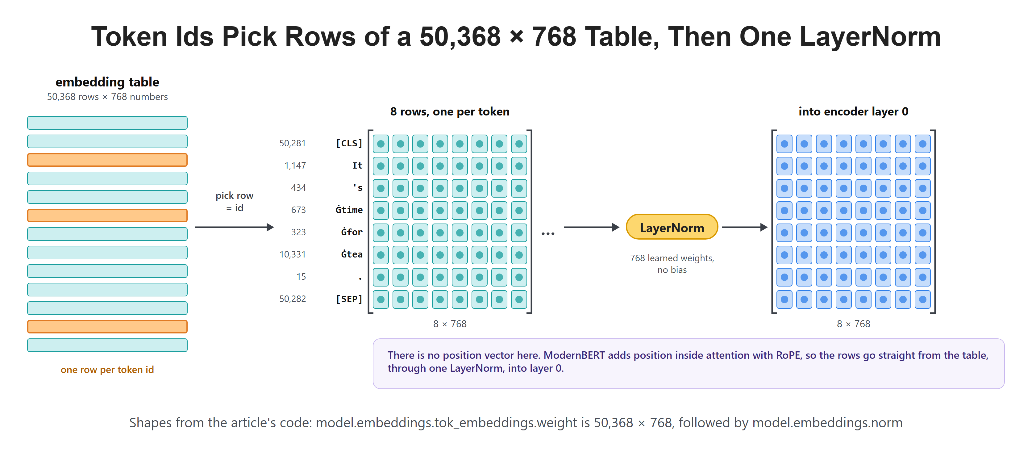
A token id is just a row number. The model keeps a table with one row of 768 numbers for each of the 50,368 tokens. To turn an id into a vector, it picks that row. ModernBERT then sends the rows through one LayerNorm before layer 0.
The figure below shows the lookup for our 8 tokens. There is no position vector in this picture. The original Transformer added one here, but ModernBERT adds position inside attention with RoPE, as we will see.
Let's check the shape of the table.
model.embeddings.tok_embeddings.weight.shapetorch.Size([50368, 768])So the table has 50,368 rows of 768 numbers, which is 38,682,624 weights. That is a quarter of the whole model. The vocabulary size 50,368 is a multiple of 64, a size GPUs handle well.
What Does LayerNorm Do?
Each encoder layer has two blocks: attention and an MLP. Before each block, the vector goes through a LayerNorm, and after each block, the block's output is added back to its input. This adding back is the residual connection. The middle panel of the architecture figure shows this order.
The numbers in a vector can drift very large or very small as they pass through 22 layers. So, here comes LayerNorm to the rescue. In simple words, LayerNorm rescales each token's vector so its numbers have a mean of 0 and a spread of 1. Then it multiplies each number by a learned weight. In the original Transformer, LayerNorm also added a learned bias. ModernBERT drops the bias.
The figure below runs LayerNorm on 4 numbers and lists the 45 places ModernBERT-base uses it.
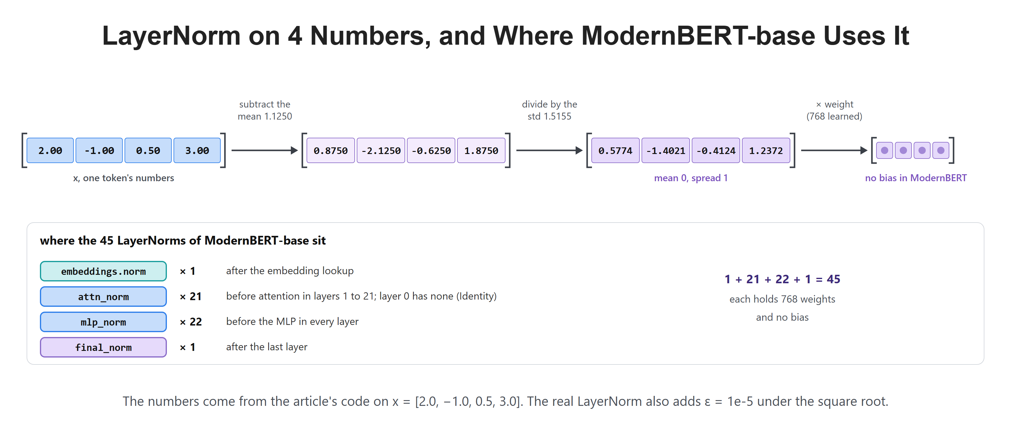
First, let's look at the norm before attention in layer 0 and layer 1.
model.layers[0].attn_norm, model.layers[1].attn_norm(Identity(), LayerNorm((768,), eps=1e-05, elementwise_affine=True))Layer 0 has no norm before attention, because its input has just come out of the embedding LayerNorm. Normalizing it twice in a row would add nothing. Every other layer has a real LayerNorm there.
Now let's do the LayerNorm math by hand on 4 numbers.
v = torch.tensor([2.0, -1.0, 0.5, 3.0])
mean, std = v.mean(), v.std(unbiased=False)
mean, std, (v - mean) / std(tensor(1.1250), tensor(1.5155), tensor([ 0.5774, -1.4021, -0.4124, 1.2372]))Here, we can see the mean is 1.1250 and the spread (the standard deviation) is 1.5155. Subtracting the mean and dividing by the spread gives 0.5774, -1.4021, -0.4124 and 1.2372. These new numbers have a mean of 0 and a spread of 1. The real LayerNorm also adds a tiny eps of 1e-5 under the square root, so it never divides by zero.
Let's confirm that the final norm has weights but no bias.
model.final_norm.weight.shape, model.final_norm.bias(torch.Size([768]), None)The weight has 768 numbers, one per position in the vector, and the bias is None. The same holds for all 45 LayerNorms in the model.
How Does Self-Attention Work?
The word "bank" means one thing in "the bank of the river" and another in "the bank approved my loan". The embedding table gives "bank" the same row both times. To tell the two apart, each token must take in information from the tokens around it. Attention is the only step in a layer that does this.
Attention gives each token three vectors, made by three learned matrices:
- Query (Q): what this token is looking for.
- Key (K): what this token offers to others.
- Value (V): the information this token hands over.
Each token's query is compared with every token's key. The scores are divided by the square root of the head size and turned into weights with softmax, so each row of weights sums to 1. Then each token's output is the weighted blend of all the values.
In a decoder like Qwen2.5, a causal mask hides every token after the current one. An encoder has no causal mask. Every token weighs every token, the ones before it and the ones after it. The only mask an encoder needs is the padding mask from the tokenizer.
The figure below runs the whole computation on 4 tokens with 8 numbers each and a head of size 4, using random weights.
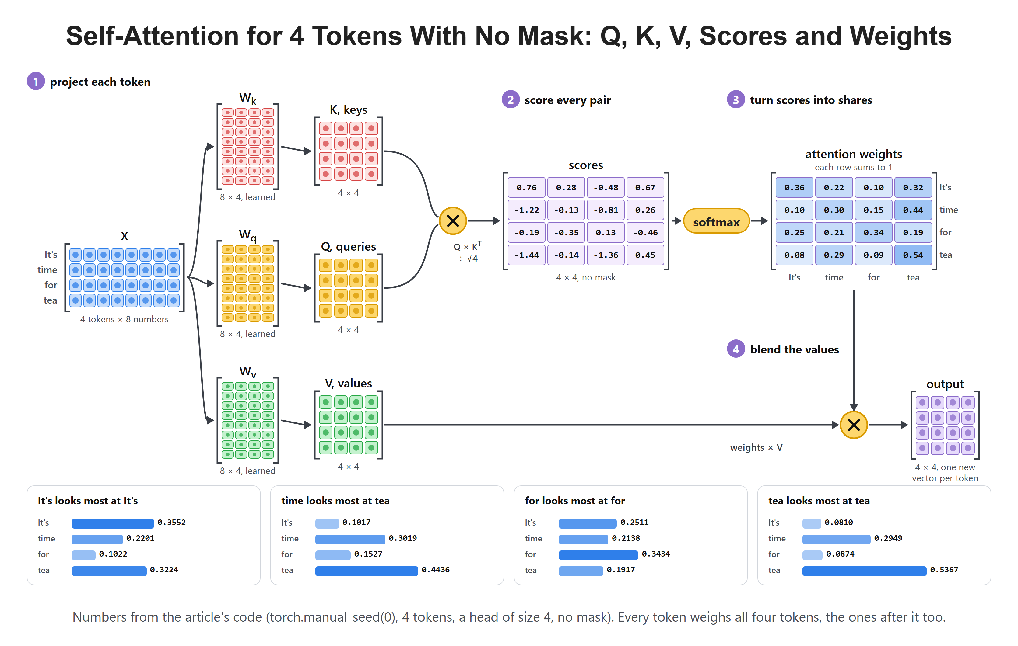
Let's see the code as below. It builds X and the three W matrices from a fixed seed, then computes the weights.
torch.manual_seed(0)
X = torch.randn(4, 8)
Wq = torch.randn(8, 4) / 8 ** 0.5
Wk = torch.randn(8, 4) / 8 ** 0.5
Wv = torch.randn(8, 4) / 8 ** 0.5

Q, K, V = X @ Wq, X @ Wk, X @ Wv
weights = torch.softmax(Q @ K.T / 4 ** 0.5, dim=-1)
weightstensor([[0.3552, 0.2201, 0.1022, 0.3224],
[0.1017, 0.3019, 0.1527, 0.4436],
[0.2511, 0.2138, 0.3434, 0.1917],
[0.0810, 0.2949, 0.0874, 0.5367]])Here, we can see a full 4 × 4 grid with no zeros. The first token puts 0.3224 on the last token, a token that comes after it. A decoder would have forced that weight to 0. Each row sums to 1.
The last step blends the values. PyTorch has a built-in function for the whole computation, so let's check our result against it.
out = weights @ V
torch.allclose(out, torch.nn.functional.scaled_dot_product_attention(Q, K, V))TrueSo our by-hand attention matches PyTorch's scaled_dot_product_attention, which also uses no mask by default.
Why Can an Encoder Look Both Ways?
A decoder writes text left to right, so it must never peek at the tokens it has not written yet. An encoder never writes. It sees the whole text from the start, so it can read in both directions. This is the real difference between the two, and it shows up clearly in the attention weights of trained models.
The figure below shows one head of each model on the same sentence. On the left is a head from Qwen2.5-0.5B, a decoder, from our Qwen2.5-0.5B teardown. On the right is a head from ModernBERT-base.
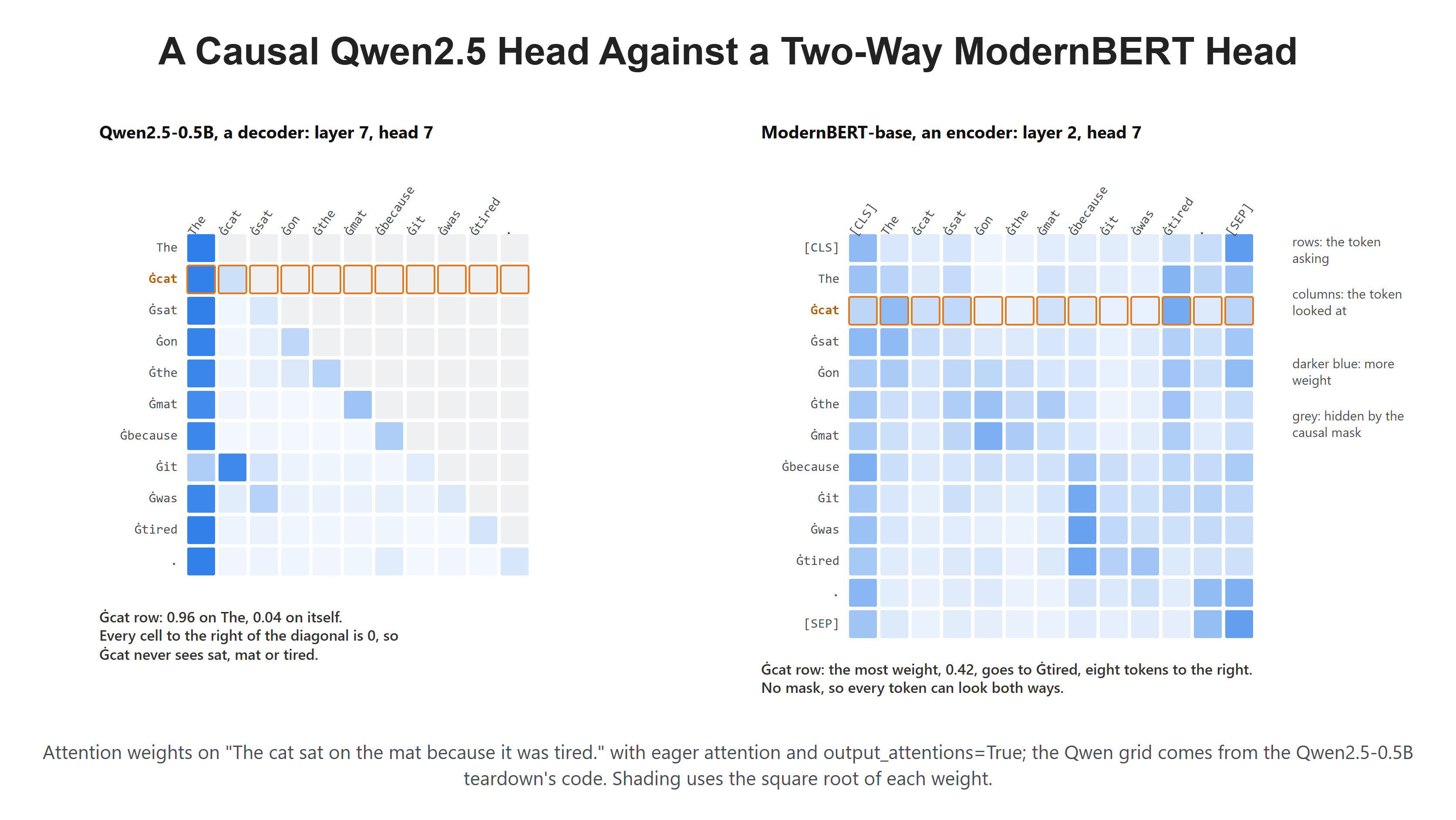
Here, we can see the Qwen grid is a triangle: everything to the right of the diagonal is 0. The ModernBERT grid is filled in everywhere. In the Ġcat row, Qwen can only weigh "The" and "cat" itself. ModernBERT puts its most weight on "tired", eight tokens later.
To read real attention weights, we switch the model to the plain "eager" attention, which can return them.
model.set_attn_implementation("eager")

x = tok("The cat sat on the mat because it was tired.", return_tensors="pt").to("cuda")
response = model(**x, output_attentions=True)
len(response.attentions), response.attentions[0].shape(22, torch.Size([1, 12, 13, 13]))We get 22 grids, one per layer. Each has shape [1, 12, 13, 13]: 1 sentence, 12 heads, and 13 tokens asking times 13 tokens looked at. The sentence has 11 tokens, plus [CLS] and [SEP].
Let's find where Ġcat looks most in layer 2, head 7.
tokens = tok.convert_ids_to_tokens(x["input_ids"][0])
A = response.attentions[2][0, 7].float().cpu()
tokens[2], tokens[A[2].argmax()], round(A[2].max().item(), 2)('Ġcat', 'Ġtired', 0.42)So the token Ġcat gives 0.42 of its attention to Ġtired, a token to its right. In a decoder, this cell would be 0.
How Does ModernBERT Make Q, K and V?
One head gives each token one way to look around. Real models run many heads side by side, so different heads can follow different links. ModernBERT-base has 12 heads, each working on 64 numbers, and 12 × 64 = 768.
The original Transformer makes Q, K and V with three separate matrices. ModernBERT fuses them into one matrix, Wqkv, which turns 768 numbers into 2,304 = 3 × 768. One large matrix multiply usually runs faster on a GPU than three small ones. The result is then cut into Q, K and V, and each of them into 12 heads.
The figure below shows that cut.
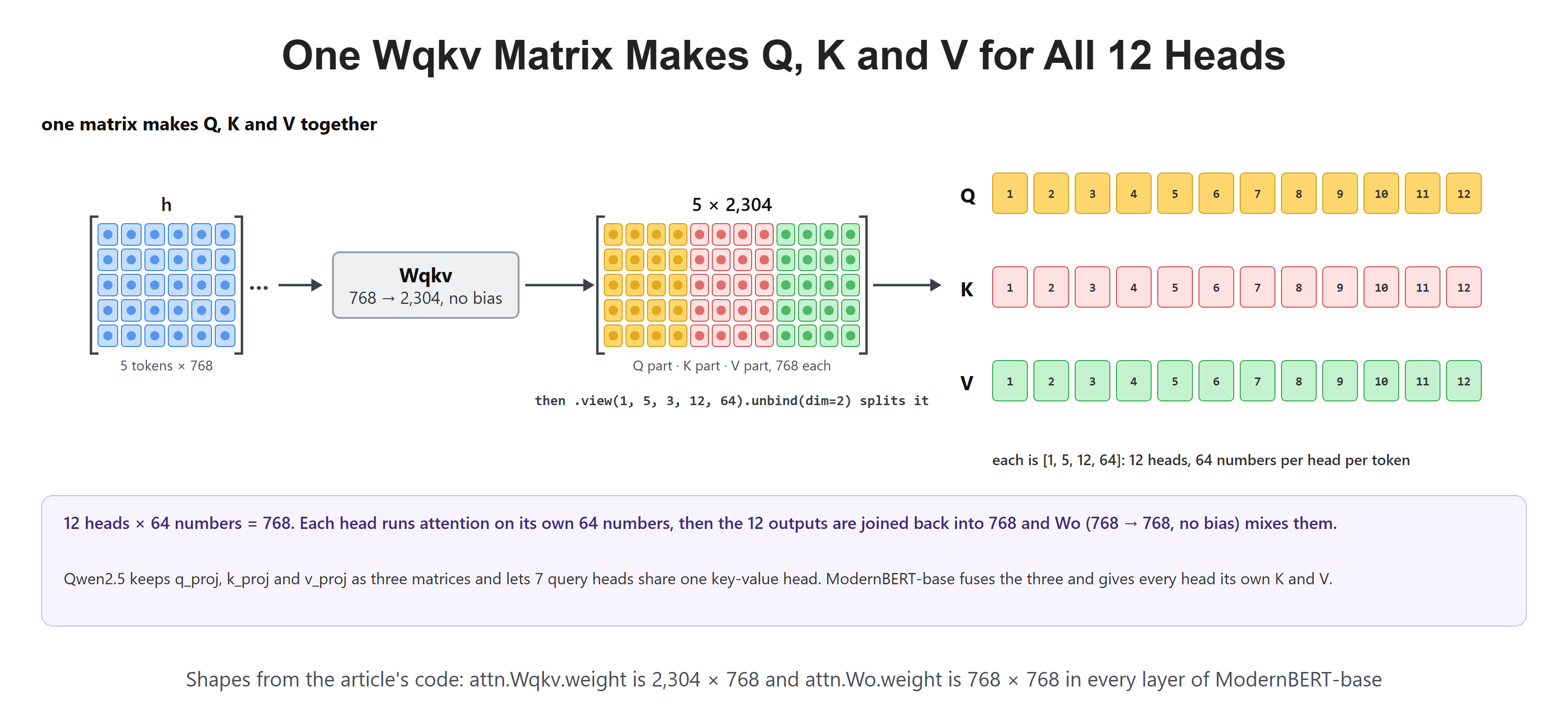
Let's check the two attention matrices of layer 0.
attn = model.layers[0].attn
attn.Wqkv.weight.shape, attn.Wo.weight.shape(torch.Size([2304, 768]), torch.Size([768, 768]))Wqkv maps 768 numbers to 2,304, and Wo maps the joined heads back from 768 to 768. PyTorch stores a Linear weight as [out, in], so the shapes read backwards.
Now let's run Wqkv on a random input of 5 tokens and cut the result the way the model does.
h = torch.randn(1, 5, 768, device="cuda")
q, k, v = attn.Wqkv(h).view(1, 5, 3, 12, 64).unbind(dim=2)
q.shape, k.shape, v.shape(torch.Size([1, 5, 12, 64]),
torch.Size([1, 5, 12, 64]),
torch.Size([1, 5, 12, 64]))Here, we can see that view splits the 2,304 numbers into 3 × 12 × 64, and unbind pulls out Q, K and V. Each one has 12 heads of 64 numbers for each of the 5 tokens. Every head has its own K and V. Qwen2.5 lets 7 query heads share one key-value head, which shrinks the cache it keeps while writing text. An encoder never writes text, so it has no such cache to shrink, and ModernBERT keeps all 12.
What Are Local and Global Attention?
Attention compares every token with every token. For n tokens, that is n × n scores per head. At 512 tokens this is fine, but ModernBERT reads up to 8,192 tokens, and 8,192 × 8,192 is over 67 million scores per head, per layer.
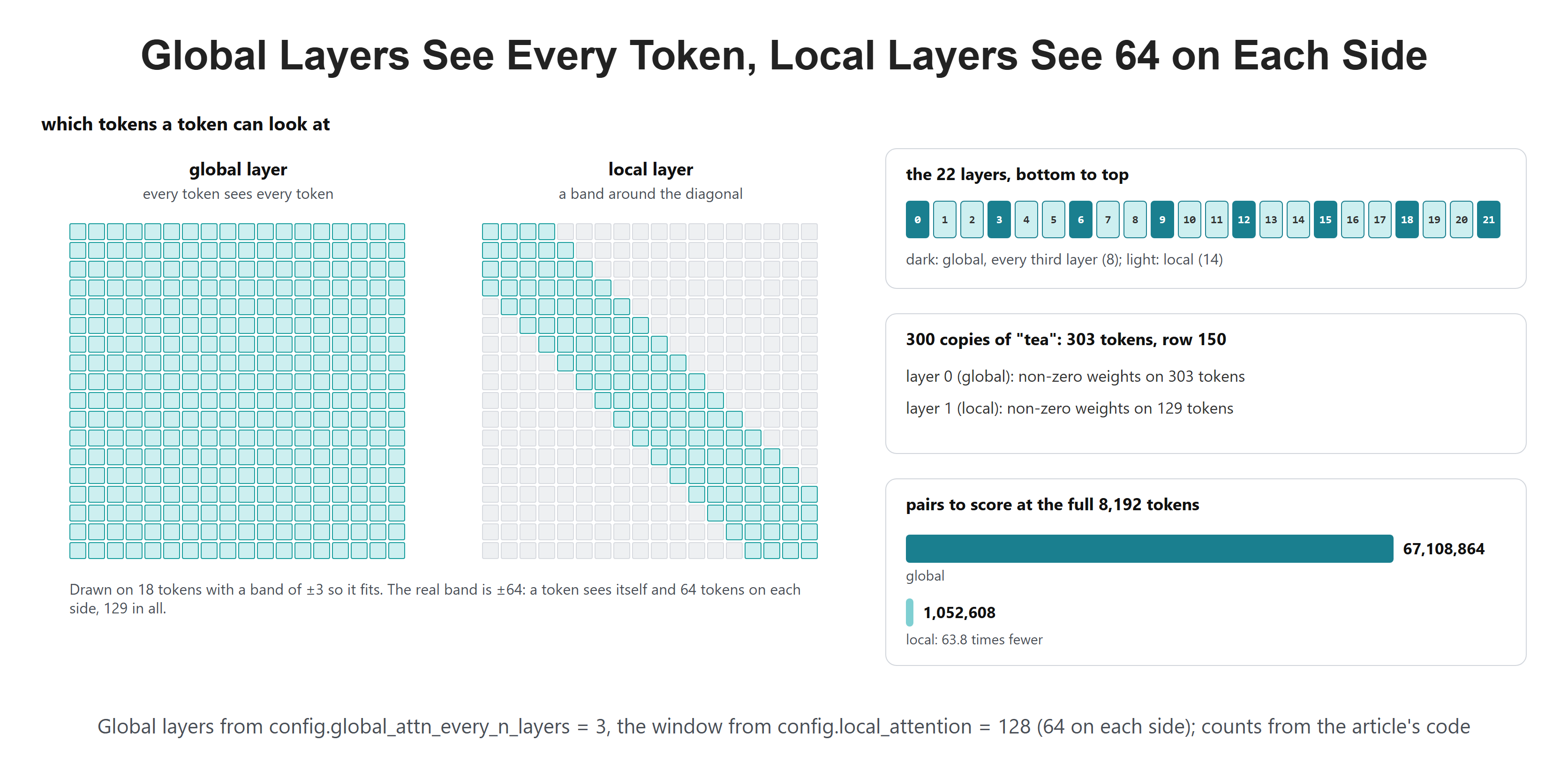
But here's the thing: most of what a word means depends on the words near it. So, here comes local attention to the rescue. In a local layer, each token looks only at the 64 tokens on each side of it and at itself, 129 tokens in all. In a global layer, each token looks at every token. ModernBERT makes every third layer global and the rest local, so information can still travel across the whole text.
The figure below shows the two kinds of mask, the order of the 22 layers and what this saves.
Let's list the global layers from the config.
[i for i, t in enumerate(config.layer_types) if t == "full_attention"][0, 3, 6, 9, 12, 15, 18, 21]So layers 0, 3, 6 and so on up to 21 are global: 8 global layers and 14 local ones. The first and the last layers are both global.
Now let's see the window in a real run. We feed 300 copies of "tea" and count how many tokens row 150 gives a non-zero weight to, in layer 0 (global) and layer 1 (local).
x = tok(" ".join(["tea"] * 300), return_tensors="pt").to("cuda")
response = model(**x, output_attentions=True)
row = 150
x["input_ids"].shape[1], (response.attentions[0][0, 0, row] > 0).sum().item(), (response.attentions[1][0, 0, row] > 0).sum().item()(303, 303, 129)Here, we can see the text has 303 tokens. In layer 0, token 150 weighs all 303 of them. In layer 1, it weighs only 129: itself and 64 on each side. Every weight outside the window is exactly 0.
Let's count how many query-key pairs each kind of layer scores at the full 8,192 tokens.
n = 8192
global_pairs = n * n
local_pairs = sum(min(i + 64, n - 1) - max(i - 64, 0) + 1 for i in range(n))
global_pairs, local_pairs, round(global_pairs / local_pairs, 1)(67108864, 1052608, 63.8)A global layer scores 67,108,864 pairs per head. A local layer scores 1,052,608, which is 63.8 times fewer. Tokens near the two ends have fewer neighbours, which is why the local count is a little under 8,192 × 129.
How Does RoPE Work With Two Bases?
Attention on its own does not know the order of the tokens. "dog bites man" and "man bites dog" contain the same tokens, so they would get the same scores. The original Transformer fixed this by adding a position vector to each embedding at the bottom of the model.
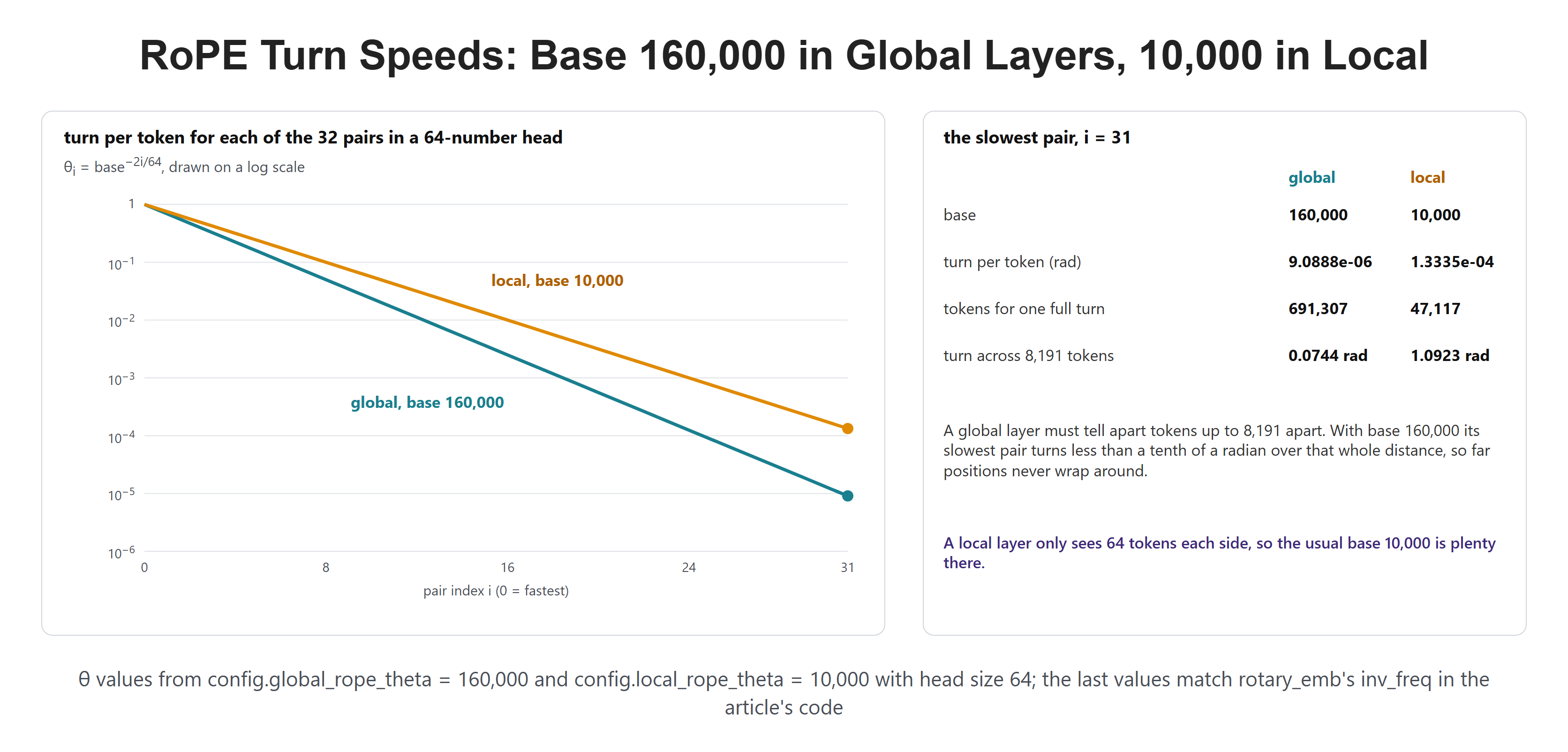
ModernBERT uses RoPE instead. In simple words, RoPE splits each query and key into pairs of numbers and turns each pair by an angle that grows with the token's position. When a query meets a key, the score then depends on how far apart the two tokens are. Each head has 64 numbers, so it has 32 pairs. Pair i turns by θi = base−2i/64 per token: the first pair turns fast and the last pair turns very slowly.
ModernBERT uses two bases. Global layers use base 160,000, so their slowest pair turns very slowly and can tell apart tokens thousands of positions apart. Local layers use base 10,000, the value from the original RoPE paper, because they only ever see 64 tokens away. Both bases come from the model's config.
The figure below plots the turn per token for all 32 pairs with both bases.
The model keeps one list of turn speeds, inv_freq, for each kind of layer. Let's read the slowest pair of each.
rope = model.rotary_emb
rope.full_attention_inv_freq[-1].item(), rope.sliding_attention_inv_freq[-1].item()(9.088847036764491e-06, 0.0001333521504420787)Here, we can see the slowest pair of a global layer turns 9.09e-06 radians per token, and that of a local layer 1.33e-04, about 15 times faster. Across 8,191 tokens, the global pair turns only 0.0744 radians, so two far-apart positions never wrap around to look the same. RoPE adds no weights at all: these speeds come from the base alone.
What Does the GeGLU MLP Do?
Attention mixes information between tokens. The MLP then works on each token alone: it reads the token's 768 numbers, widens them, reshapes them and brings them back to 768.
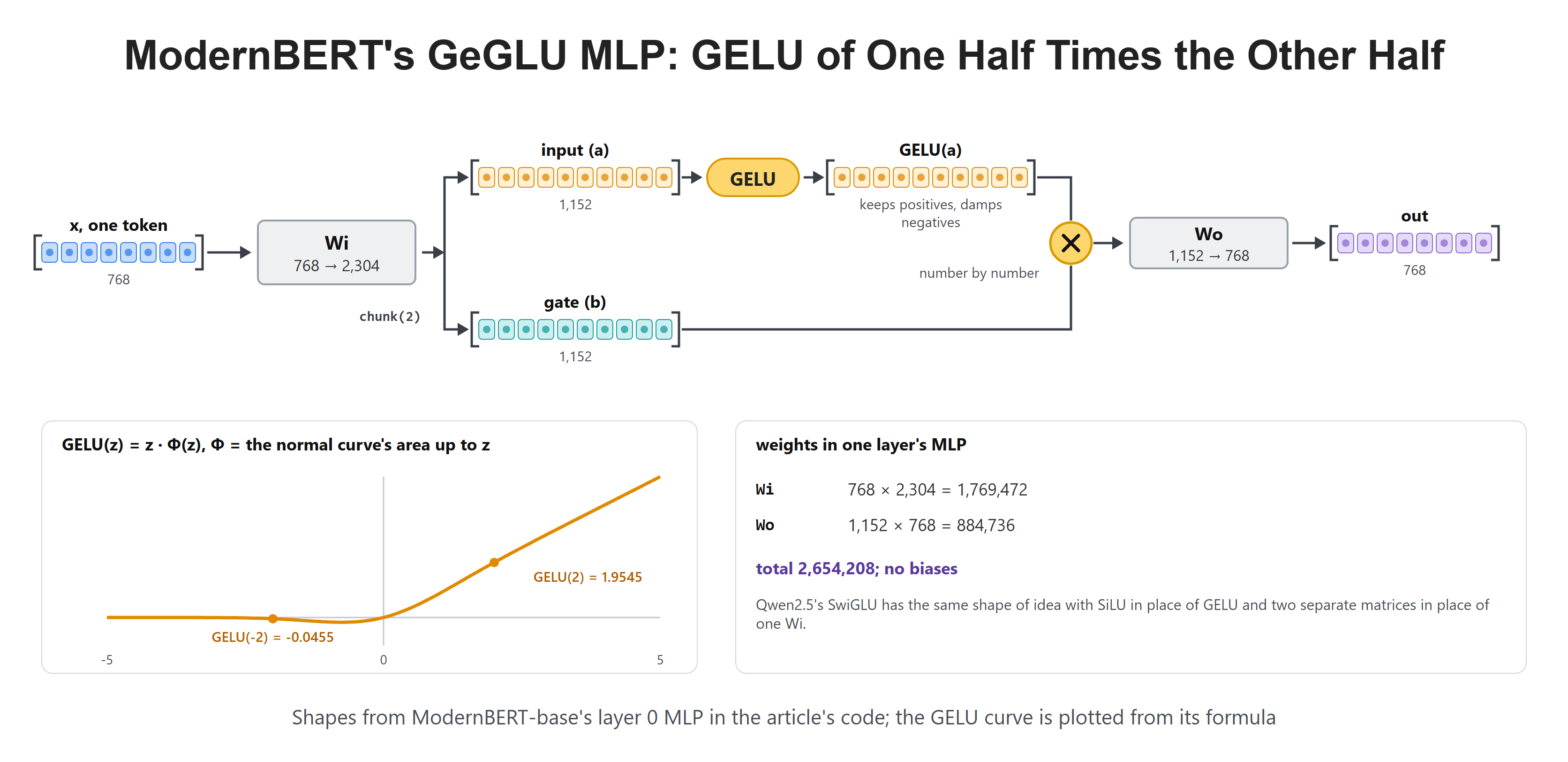
The original Transformer's MLP is two matrices with a ReLU between them. ModernBERT uses a GeGLU MLP. In simple words, Wi makes two vectors of 1,152 numbers. The first, the input, goes through GELU. The second, the gate, multiplies it number by number. So the gate decides how much of each GELU output passes through. Then Wo brings the 1,152 numbers back to 768.
The figure below shows the flow, the GELU curve and the weights in one MLP.
Let's check the shapes of the two MLP matrices.
mlp = model.layers[0].mlp
mlp.Wi.weight.shape, mlp.Wo.weight.shape(torch.Size([2304, 768]), torch.Size([768, 1152]))Wi maps 768 numbers to 2,304, which is 2 × 1,152, and Wo maps 1,152 back to 768.
Now let's split the output of Wi by hand and check it against the real MLP.
h = torch.randn(1, 768, device="cuda")
a, b = mlp.Wi(h).chunk(2, dim=-1)
a.shape, torch.allclose(mlp.Wo(mlp.act(a) * b), mlp(h))(torch.Size([1, 1152]), True)Here, we can see chunk(2) cuts the 2,304 numbers into two halves of 1,152. Wo(GELU(a) * b) gives the same result as the model's own MLP, so this one line is the whole GeGLU.
Let's see what GELU does to three numbers.
torch.nn.functional.gelu(torch.tensor([-2.0, 0.0, 2.0]))tensor([-0.0455, 0.0000, 1.9545])GELU keeps 2.0 almost as it is, 1.9545, and squeezes -2.0 to almost zero, -0.0455. It works like ReLU with a smooth bend near 0. Qwen2.5's SwiGLU follows the same plan with SiLU in place of GELU.
Where Do the 149M Parameters Sit?
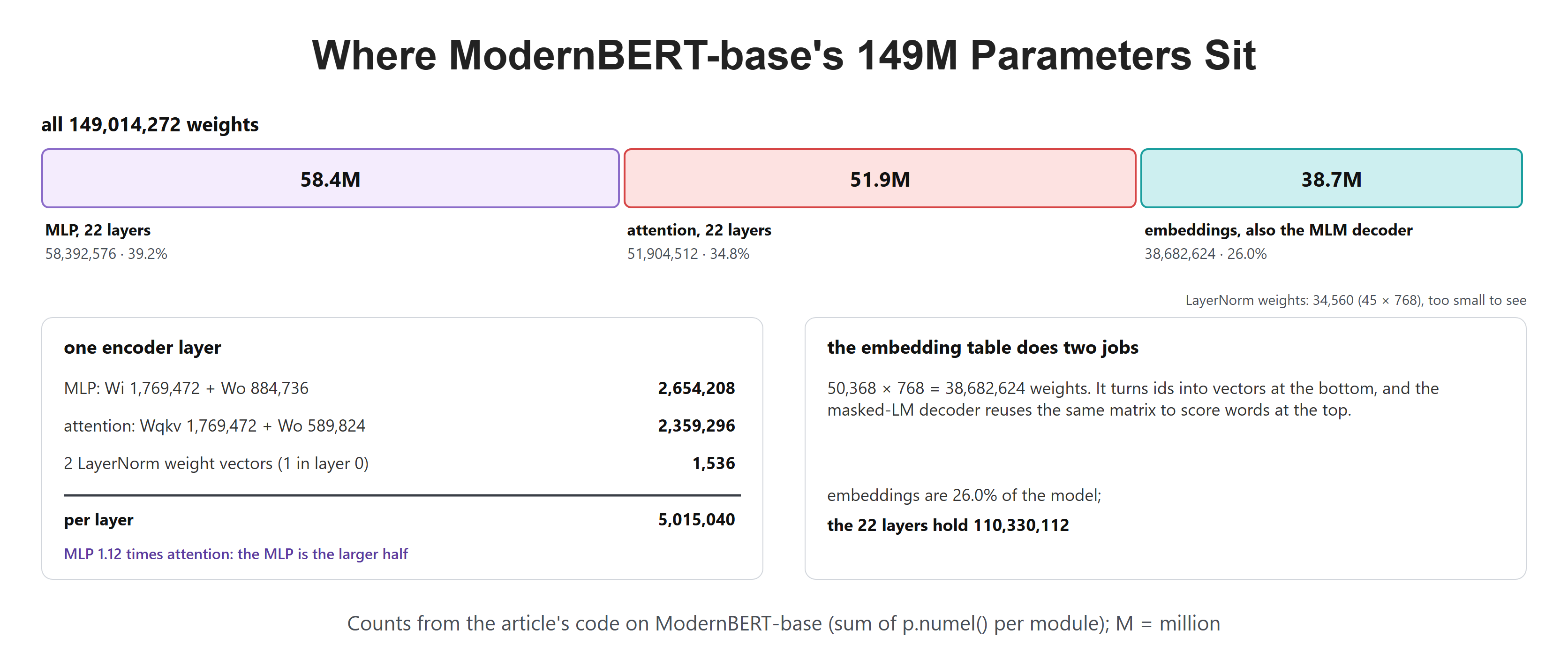
Now that we have seen every part, let's count the weights. The figure below splits all 149,014,272 of them.
Let's count attention and the MLP in one layer.
layer = model.layers[1]
sum(p.numel() for p in layer.attn.parameters()), sum(p.numel() for p in layer.mlp.parameters())(2359296, 2654208)Attention holds 2,359,296 weights: Wqkv has 768 × 2,304 = 1,769,472 and Wo has 768 × 768 = 589,824. The MLP holds 2,654,208: Wi has 768 × 2,304 = 1,769,472 and Wo has 1,152 × 768 = 884,736. So the MLP is a little larger.
Now let's count the embedding table and the whole model.
embeddings = model.embeddings.tok_embeddings.weight.numel()
total = sum(p.numel() for p in model.parameters())
embeddings, total(38682624, 149014272)Let me tabulate the full split for your better understanding.
| Part | Weights | Share |
|---|---|---|
| MLP, 22 layers | 58,392,576 | 39.2% |
| Attention, 22 layers | 51,904,512 | 34.8% |
| Embedding table | 38,682,624 | 26.0% |
| LayerNorms (45 × 768) | 34,560 | 0.02% |
| Total | 149,014,272 | 100% |
Here, we can see that the 22 layers hold 110,330,112 weights, and the embedding table holds a quarter of the model. In float32, each weight takes 4 bytes, so the whole model takes 568 MB.
How Does an Encoder Learn?
A decoder learns by guessing the next token. An encoder sees the whole text at once, so guessing the next token would be too easy: the answer is already in the input. So, ModernBERT learns by guessing hidden tokens instead. During training, some tokens are replaced with [MASK], and the model must guess what was there from the words on both sides. This is masked language modelling.
Filling in a [MASK]
The trained model can still fill in blanks, and the fill-mask pipeline shows this directly. The figure below shows its top 5 guesses for two sentences.
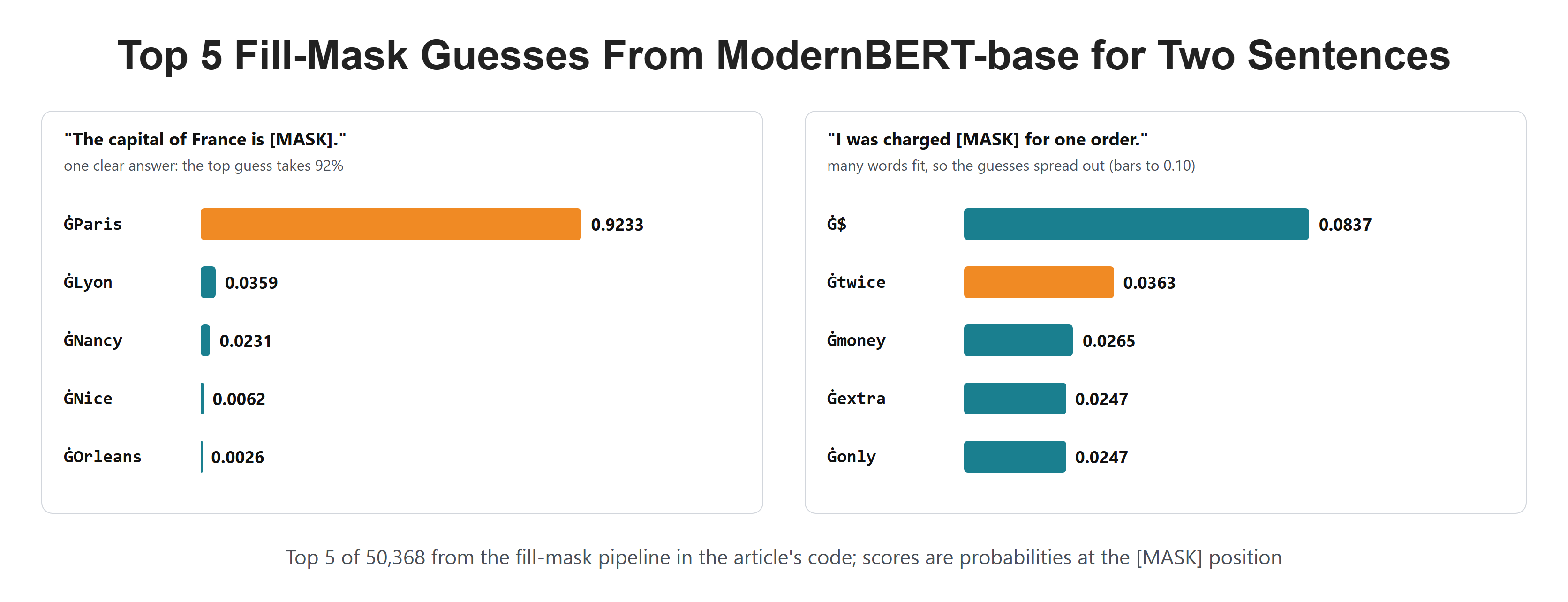
Let's start with a sentence that has one clear answer.
fill = pipeline("fill-mask", model=MODEL, device_map="cuda")

fill("The capital of France is [MASK].")[{'score': 0.9233400225639343, 'token': 7785, 'token_str': ' Paris', 'sequence': 'The capital of France is Paris.'}, {'score': 0.0359475240111351, 'token': 42268, 'token_str': ' Lyon', 'sequence': 'The capital of France is Lyon.'}, {'score': 0.023051084950566292, 'token': 23397, 'token_str': ' Nancy', 'sequence': 'The capital of France is Nancy.'}, {'score': 0.006168763153254986, 'token': 29902, 'token_str': ' Nice', 'sequence': 'The capital of France is Nice.'}, {'score': 0.0025843221228569746, 'token': 20159, 'token_str': ' Orleans', 'sequence': 'The capital of France is Orleans.'}]Here, we can see " Paris" gets 0.9233 of the probability, and the next four guesses are all French cities. Now let's try a sentence where many words fit.
fill("I was charged [MASK] for one order.")[{'score': 0.08371848613023758, 'token': 370, 'token_str': ' [{'score': 0.08371848613023758, 'token': 370, 'token_str': ' $', 'sequence': 'I was charged $ for one order.'}, {'score': 0.036309946328401566, 'token': 7019, 'token_str': ' twice', 'sequence': 'I was charged twice for one order.'}, {'score': 0.026476478204131126, 'token': 2583, 'token_str': ' money', 'sequence': 'I was charged money for one order.'}, {'score': 0.024666978046298027, 'token': 4465, 'token_str': ' extra', 'sequence': 'I was charged extra for one order.'}, {'score': 0.02466323785483837, 'token': 760, 'token_str': ' only', 'sequence': 'I was charged only for one order.'}]#x27;, 'sequence': 'I was charged $ for one order.'}, {'score': 0.036309946328401566, 'token': 7019, 'token_str': ' twice', 'sequence': 'I was charged twice for one order.'}, {'score': 0.026476478204131126, 'token': 2583, 'token_str': ' money', 'sequence': 'I was charged money for one order.'}, {'score': 0.024666978046298027, 'token': 4465, 'token_str': ' extra', 'sequence': 'I was charged extra for one order.'}, {'score': 0.02466323785483837, 'token': 760, 'token_str': ' only', 'sequence': 'I was charged only for one order.'}]This time, the top guess gets only 0.0837. " twice" comes second with 0.0363, and " money", " extra" and " only" follow. Many words fit the blank, so the probability spreads out.
The Masked-LM Head
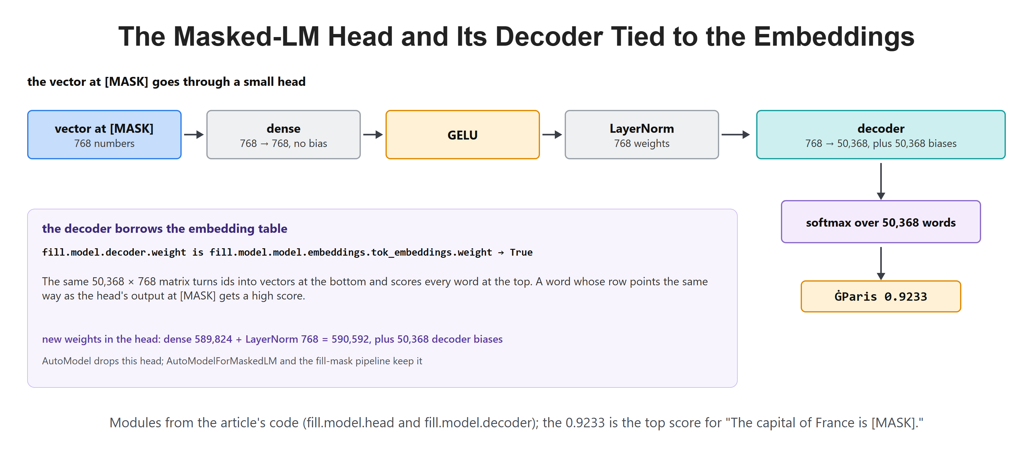
AutoModel stops at one vector per token. To score words, the pipeline loads the model with a small head on top. The head takes the vector at [MASK], passes it through a dense layer, GELU and a LayerNorm, and then a decoder turns 768 numbers into 50,368 scores, one per vocabulary entry.
The figure below shows the head, and the trick in its decoder.
Let's print the two parts.
fill.model.head, fill.model.decoder(ModernBertPredictionHead(
(dense): Linear(in_features=768, out_features=768, bias=False)
(act): GELUActivation()
(norm): LayerNorm((768,), eps=1e-05, elementwise_affine=True)
),
Linear(in_features=768, out_features=50368, bias=True))Here, we can see the head and the decoder. The decoder is the only Linear in the whole model with a bias. A decoder from 768 to 50,368 would need 38,682,624 weights, the same count as the embedding table. Let's check whether it is the embedding table.
fill.model.decoder.weight is fill.model.model.embeddings.tok_embeddings.weightTrueSo the decoder's weight is the very same tensor as the embedding table. This is called weight tying. One matrix turns ids into vectors at the bottom and scores words at the top. A word gets a high score when its embedding row points the same way as the head's output at [MASK].
How Training Picks Tokens to Mask
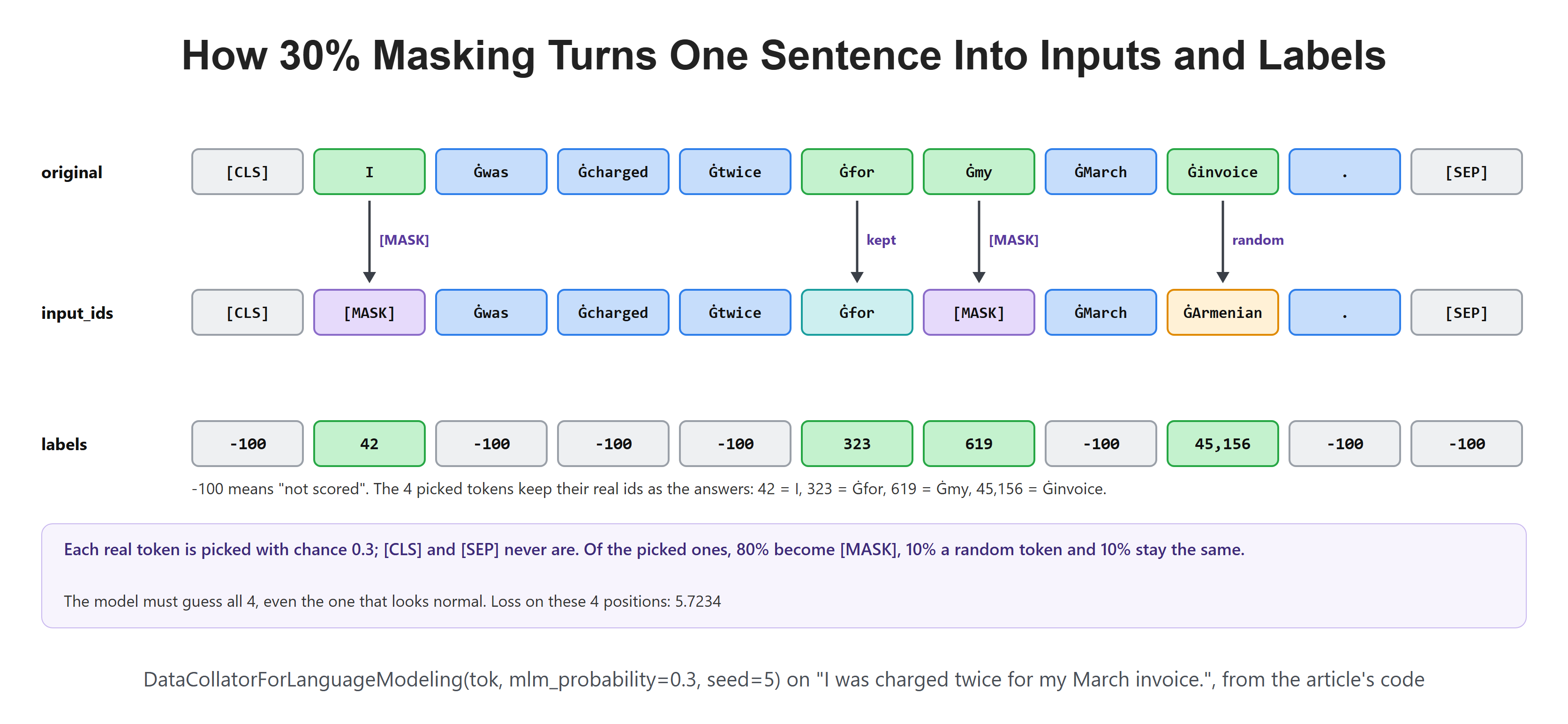
During training, a data collator hides the tokens. ModernBERT uses a masking rate of 30%. Each real token is picked with a chance of 0.3, and [CLS] and [SEP] are never picked. Of the picked tokens, 80% become [MASK], 10% become a random token and 10% stay the same. This mix is the recipe from the original BERT, and it is the default of Hugging Face's collator. The random and unchanged tokens teach the model that any token might be wrong, not only the ones marked [MASK].
The figure below shows one run of the collator on one sentence.
Let's see the code as below. We fix the seed so the same tokens are picked every time.
from transformers import DataCollatorForLanguageModeling

collator = DataCollatorForLanguageModeling(tok, mlm_probability=0.3, seed=5)
batch = collator([tok("I was charged twice for my March invoice.")])
tok.convert_ids_to_tokens(batch["input_ids"][0])['[CLS]', '[MASK]', 'Ġwas', 'Ġcharged', 'Ġtwice', 'Ġfor', '[MASK]', 'ĠMarch', 'ĠArmenian', '.', '[SEP]']Here, we can see all three kinds of pick. "I" and "my" became [MASK]. "invoice" became the random token ĠArmenian. The fourth pick, "for", stayed the same, so we cannot see it in the input. The labels show it.
batch["labels"][0]tensor([ -100, 42, -100, -100, -100, 323, 619, -100, 45156, -100,
-100])The labels hold the real id at each of the 4 picked positions: 42 for "I", 323 for "for", 619 for "my" and 45,156 for "invoice". Every other position holds -100, which tells the loss to skip it. So the model is scored only on the tokens it had to guess. This sentence got 4 picks out of 9 real tokens, because each pick is a coin flip and short texts vary.
Let's run the masked batch through the model with its labels.
response = fill.model(input_ids=batch["input_ids"].to("cuda"), labels=batch["labels"].to("cuda"))
response.losstensor(5.7234, device='cuda:0')The loss is the cross-entropy averaged over the 4 picked positions: 5.7234. It is high because guessing "I", "my" and "invoice" from this little context is hard. Training lowers this number over trillions of tokens.
For an easy blank, the loss is small. Let's build the labels by hand for the Paris sentence.
x = tok("The capital of France is [MASK].", return_tensors="pt").to("cuda")
labels = torch.full_like(x["input_ids"], -100)
labels[x["input_ids"] == tok.mask_token_id] = tok.convert_tokens_to_ids("ĠParis")

response = fill.model(**x, labels=labels)
response.losstensor(0.0798, device='cuda:0')Here, we can see a loss of 0.0798, which is minus the log of 0.9233, the probability the model gave Paris. A confident right guess costs almost nothing.
Why Does the Same Word Get Different Vectors?
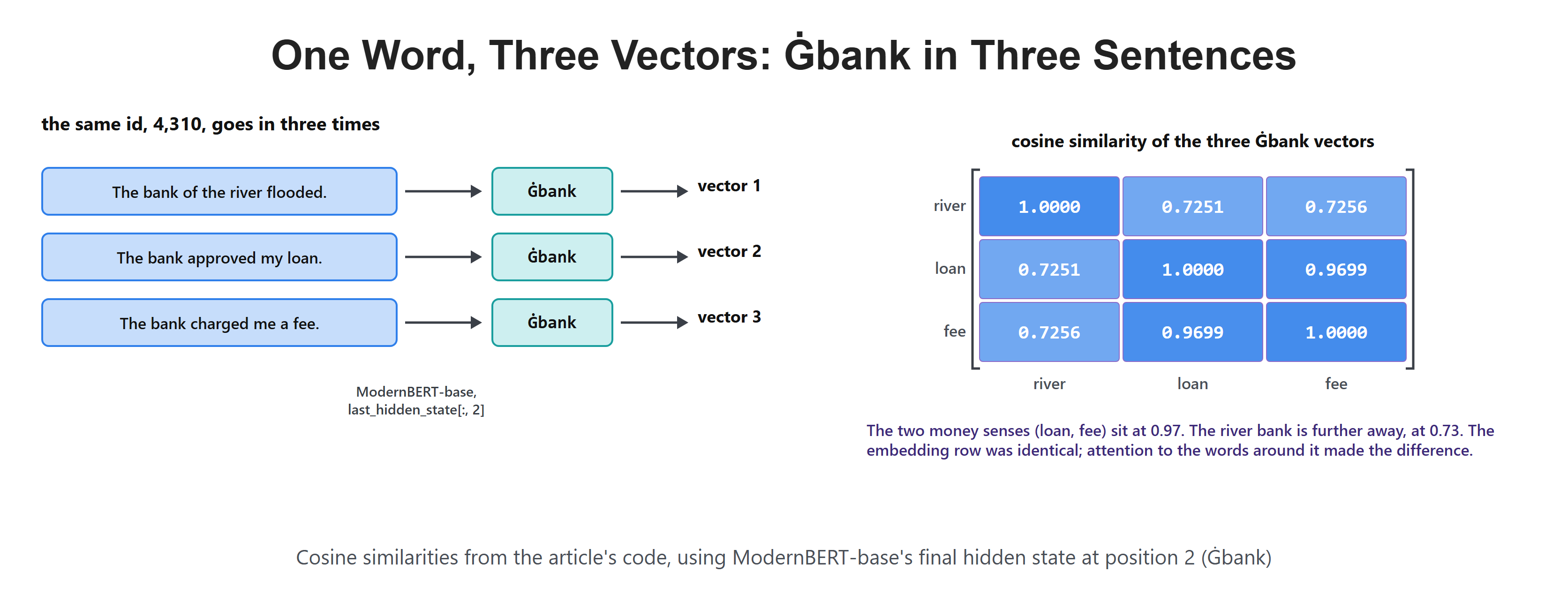
We started the attention section with the word "bank". Now let's check that the trained encoder really tells its meanings apart. We run three sentences, each with "bank" at the same position, and compare the final vectors at that position.
The figure below shows the three sentences and the cosine similarity of the three "bank" vectors. A cosine of 1 means two vectors point the same way.
First, let's confirm that position 2 is Ġbank in all three.
texts = ["The bank of the river flooded.", "The bank approved my loan.", "The bank charged me a fee."]

x = tok(texts, return_tensors="pt", padding=True).to("cuda")
tok.convert_ids_to_tokens(x["input_ids"][:, 2])['Ġbank', 'Ġbank', 'Ġbank']All three start from the same token, id 4,310, and so from the same embedding row. Let's compare the final vectors.
bank = model(**x).last_hidden_state[:, 2]
torch.cosine_similarity(bank[:, None], bank[None], dim=-1)tensor([[1.0000, 0.7251, 0.7256],
[0.7251, 1.0000, 0.9699],
[0.7256, 0.9699, 1.0000]], device='cuda:0')Here, we can see the two money senses, "approved my loan" and "charged me a fee", sit at 0.9699. The river bank is further from both, at 0.7251 and 0.7256. The 22 layers of two-way attention pulled the same starting row apart according to its neighbours on both sides.
How Do We Get One Vector per Text?
The encoder gives one vector per token. But to classify a support ticket or search for similar texts, we need one vector per text. So we pool the token vectors into one.
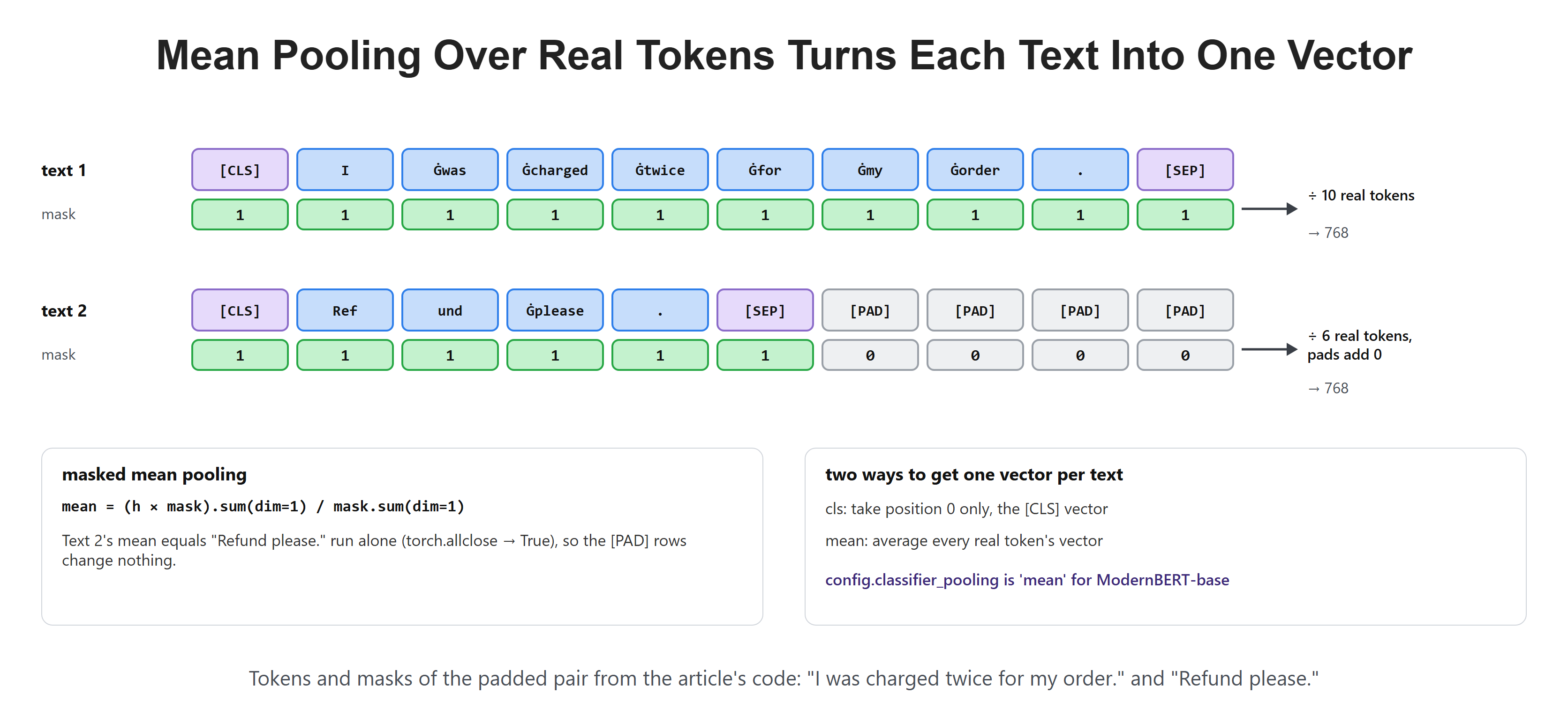
There are two common ways. CLS pooling takes only the vector at position 0, the [CLS] token. Mean pooling averages the vectors of all real tokens. With padding, the mean must skip the [PAD] tokens, or the pads would pull the average around. ModernBERT-base uses mean pooling.
The figure below shows mean pooling on a padded batch of two texts.
Let's look at the shape of the encoder's output for one text.
x = tok("I was charged twice for my order.", return_tensors="pt").to("cuda")
response = model(**x)
response.last_hidden_state.shapetorch.Size([1, 10, 768])We get 10 vectors of 768 numbers: 8 tokens of text, plus [CLS] and [SEP]. Averaging over the tokens gives one vector.
response.last_hidden_state.mean(dim=1).shapetorch.Size([1, 768])With one text, there is no padding, so a plain mean works. With a padded batch, we multiply by the mask before summing and divide by the number of real tokens.
pair = tok(["I was charged twice for my order.", "Refund please."], return_tensors="pt", padding=True).to("cuda")
h = model(**pair).last_hidden_state
mask = pair["attention_mask"].unsqueeze(-1)
mean = (h * mask).sum(dim=1) / mask.sum(dim=1)
alone = model(**tok("Refund please.", return_tensors="pt").to("cuda")).last_hidden_state.mean(dim=1)
mean.shape, torch.allclose(mean[1], alone[0], atol=1e-4)(torch.Size([2, 768]), True)Here, we can see one vector per text. The pooled vector of "Refund please." inside the padded batch matches the same text run alone, so the 4 [PAD] tokens changed nothing.
The model's config says which pooling its classification head uses.
config.classifier_pooling'mean'So ModernBERT-base pools with the mean, the same masked mean we just wrote.
How Do We Put a Classifier on Top?
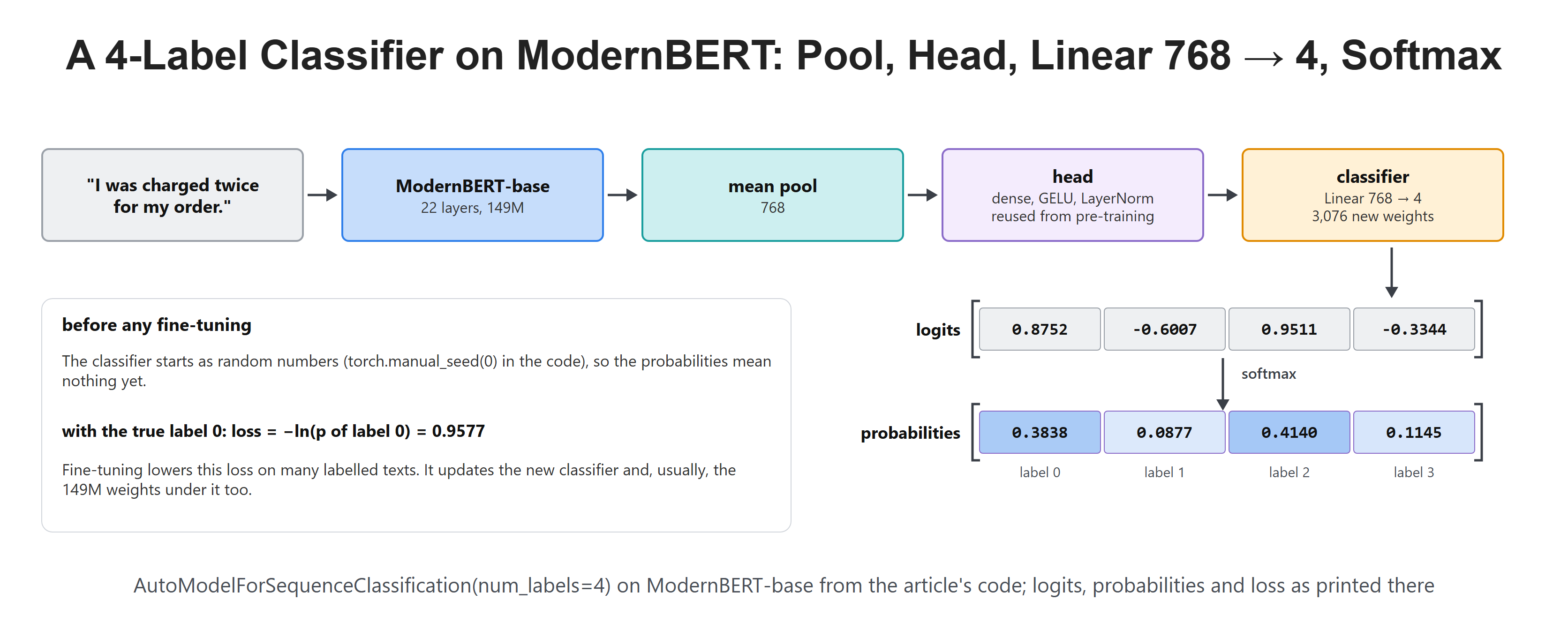
To sort texts into classes, we put a small classifier on the pooled vector. AutoModelForSequenceClassification builds the whole thing: the encoder, mean pooling, a head and a final Linear layer with one score per label. We use 4 labels, like four support-ticket teams.
The figure below shows the full path from a text to its label probabilities.
Let's load the model with 4 labels. We fix the seed, because the final layer starts with random weights.
torch.manual_seed(0)
clf = AutoModelForSequenceClassification.from_pretrained(MODEL, num_labels=4, device_map="cuda")
clf.head, clf.classifier(ModernBertPredictionHead(
(dense): Linear(in_features=768, out_features=768, bias=False)
(act): GELUActivation()
(norm): LayerNorm((768,), eps=1e-05, elementwise_affine=True)
),
Linear(in_features=768, out_features=4, bias=True))Here, we can see the same ModernBertPredictionHead as in the masked-LM model: a dense layer, GELU and a LayerNorm. It is loaded with its trained weights from pre-training. Only classifier is new: a Linear from 768 numbers to 4 scores.
sum(p.numel() for p in clf.classifier.parameters())3076The new layer has 768 × 4 = 3,072 weights plus 4 biases, 3,076 in all. Let's run our sentence through it.
clf(**x).logitstensor([[ 0.8752, -0.6007, 0.9511, -0.3344]], device='cuda:0')We get 4 raw scores, the logits. Softmax turns them into probabilities.
clf(**x).logits.softmax(dim=-1)tensor([[0.3838, 0.0877, 0.4140, 0.1145]], device='cuda:0')The probabilities sum to 1, but they mean nothing yet: the classifier is still random. Let's say the true label is 0 and compute the loss.
clf(**x, labels=torch.tensor([0], device="cuda")).losstensor(0.9577, device='cuda:0')The loss is 0.9577, which is minus the log of 0.3838, the probability of label 0. Fine-tuning shows the model many labelled texts and lowers this loss. It trains the new classifier and, usually, the 149M weights under it too.
Conclusion
This is how ModernBERT-base works. We started with text, wrapped it in [CLS] and [SEP], and looked up its tokens in a 50,368 × 768 table. We built self-attention by hand with no mask and saw a trained ModernBERT head look both ways, where a decoder head cannot. We followed the vectors through 22 encoder layers, each one a LayerNorm, attention from one fused Wqkv with RoPE, a second LayerNorm and a GeGLU MLP, joined by residual adds, with every third layer global and the rest local. Finally, we saw how the encoder learns by filling in masked tokens, and how mean pooling and a small head turn its vectors into a classifier.
Key takeaways:
- An encoder has no causal mask, so every token weighs the tokens on both sides, and the only mask it needs is for padding.
- ModernBERT-base keeps the encoder plan of the original Transformer but swaps the parts: LayerNorm without bias, RoPE, local and global attention and GeGLU.
- 8 of the 22 layers are global; the other 14 see only 64 tokens on each side, which scores 63.8 times fewer pairs at 8,192 tokens.
- Global layers use RoPE base 160,000 and local layers use base 10,000, and RoPE adds no weights.
- The model learns by guessing 30% of the tokens, and its masked-LM decoder reuses the 38.7M-weight embedding table.
Next steps:
- Read Qwen2.5-0.5B Architecture Teardown: Every Layer With Real Code to see the decoder side, layer by layer.
- Read Encoder-Only vs Decoder-Only vs Encoder-Decoder Transformers for the three families side by side.
- Read RoPE: Rotary Position Embeddings and Long Context for more on rotary positions.
- Read Transformer Architecture and Tokenization Explained for the basics of tokens, embeddings and attention.