Transformers are the engine behind almost every modern language model, from ChatGPT to Gemini. In simple words, a Transformer is a neural network that is very good at reading text and working out how each word relates to all the others. This one design is what made today's AI boom possible.
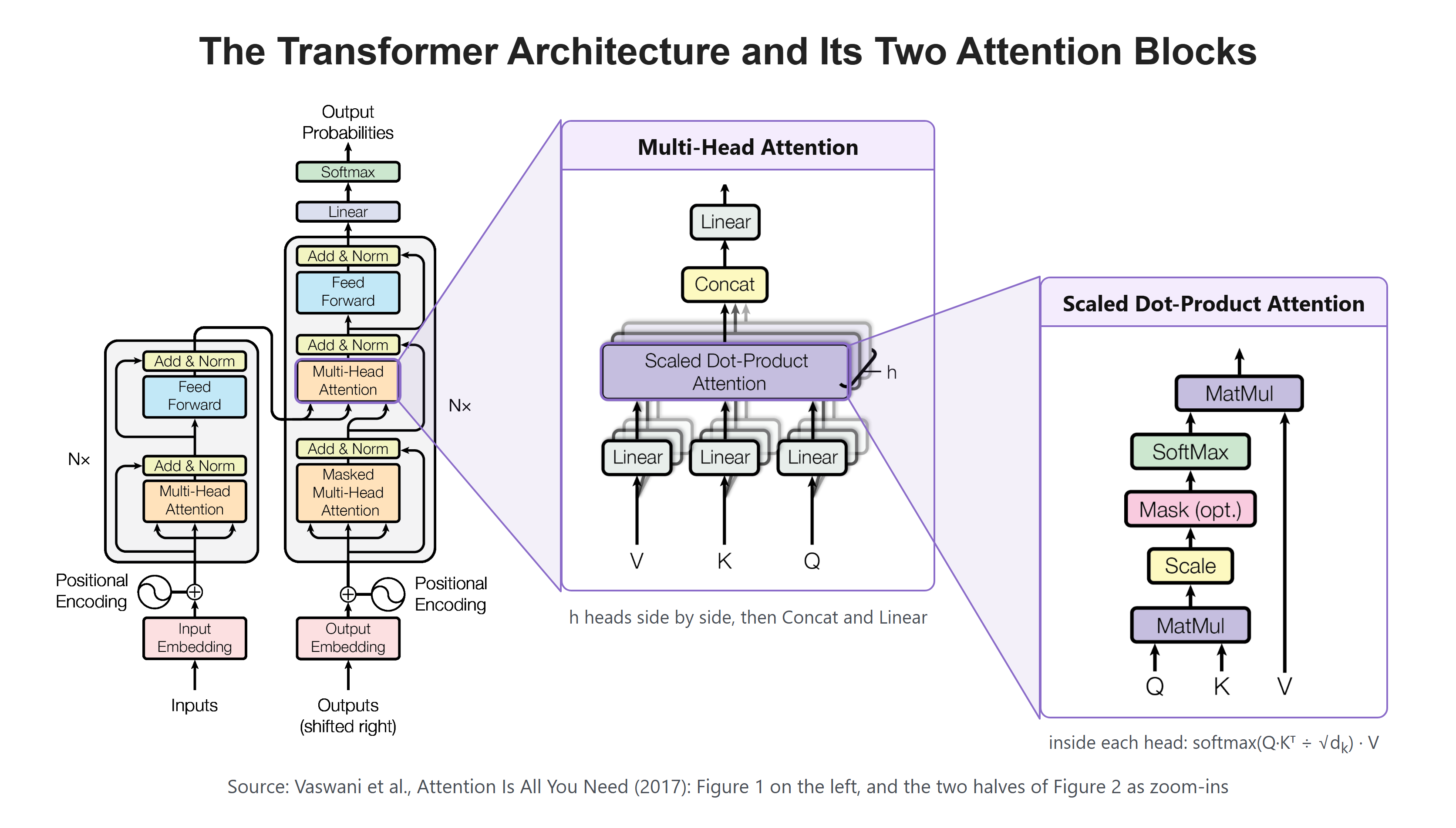
Here, we can see the original Transformer figures from the 2017 paper "Attention Is All You Need" by Vaswani et al. On the left is the whole model: the encoder tower and the decoder tower. The middle panel zooms into one Multi-Head Attention block. It runs h attention heads side by side, joins their outputs with Concat, and passes the result through a Linear layer. The right panel zooms one level deeper, into the Scaled Dot-Product Attention that runs inside each head. It multiplies the queries Q by the keys K, scales the scores, optionally masks them, turns them into weights with SoftMax, and uses those weights to blend the values V. In this lesson, we will meet these pieces one by one: the embeddings at the bottom, the positional encoding added to them, and the attention blocks inside both towers.
But a model cannot read letters the way we do. It only understands numbers. So the very first job is always the same: turn our text into numbers, and do it in a smart way. That is what this whole module is about.
In this lesson, we will follow one sentence on its full journey through a Transformer. First we chop text into tokens. Then we turn those tokens into vectors called embeddings. Next we watch attention let every token look at every other token. And finally we meet the three great families of Transformers: encoder-only, decoder-only, and encoder-decoder.
Prerequisites: intermediate Python and a basic feel for how neural networks train (loss, gradients, overfitting). We use Hugging Face and the tokenizers library for the small code demos.
Why Can't a Model Just Read Words?
Let's start with the very first problem. A neural network only does math on numbers. It cannot take the raw text "unbelievable" and work with it directly. So we need a step that turns text into numbers. This step is called tokenization.
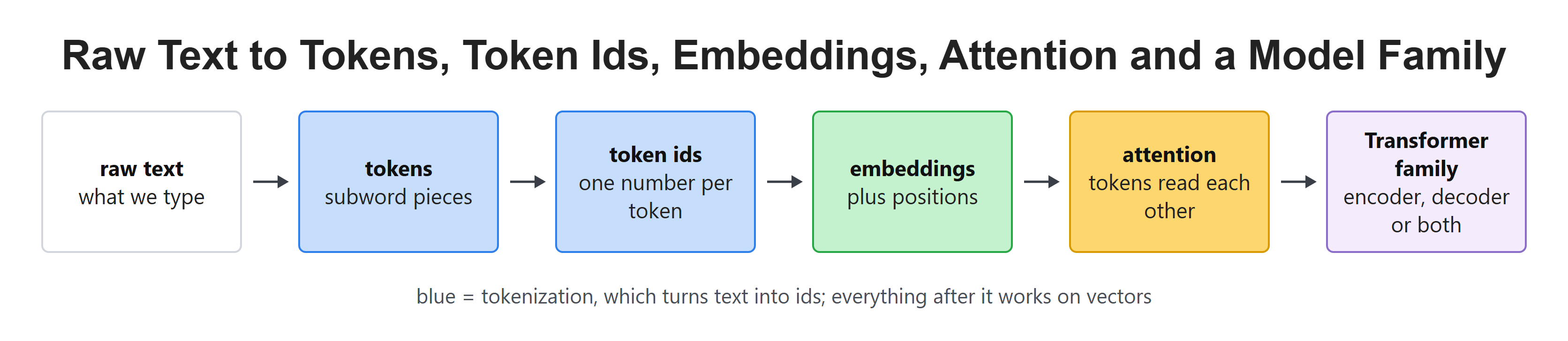
In simple words, tokenization chops text into small pieces called tokens, and gives each token a number called a token id. A token can be a whole word, a part of a word, or even a single character. The model never sees the letters. It only sees the ids.
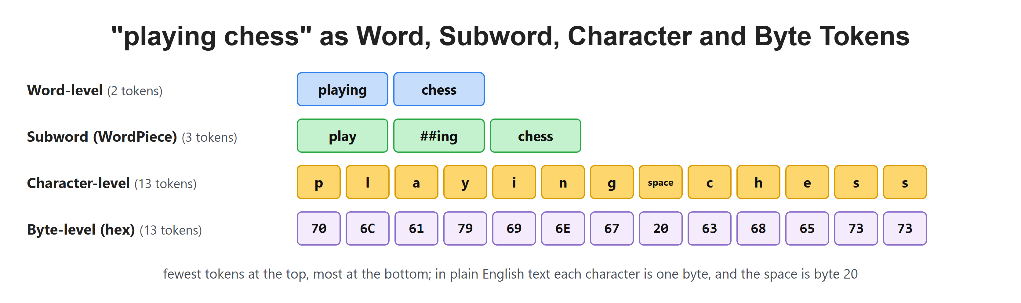
So the real question is not whether to split the text, but where to make the cuts. Let's look at our choices.
What Counts as a Token?
There are a few ways to cut text into tokens, and each one is a trade-off.
The simplest idea is word-level: every word is one token. This feels natural, but it has a big problem. The vocabulary grows huge, and any new word the model never saw, like a typo or a rare name, becomes an unknown token with no meaning.
The opposite idea is character-level: every single letter is a token. Now the vocabulary is tiny and nothing is ever unknown. But a short sentence becomes a very long list of tokens, and the model has to work much harder to see whole words.
Subword tokenization sits in the middle, and it is what almost every modern model uses. Common words stay whole, while rare words are split into smaller known pieces. So "unbelievable" might become un, believ, and able. We get a reasonable vocabulary size and we never get stuck on a new word.
Byte-level goes one step below characters. It works on the raw bytes of the text, so it can handle any language, any emoji, and any symbol without ever failing. This is the safety net that catches everything else.
How Does Byte-Pair Encoding (BPE) Build Its Vocabulary?
The most popular subword method is Byte-Pair Encoding, or BPE. The idea is beautiful and simple.
We start with the smallest pieces, single characters. Then we look at all our text and find the pair of pieces that sit next to each other most often. We glue that pair into one new token. Then we repeat: find the next most common pair, glue it, and so on. Each round builds a slightly bigger piece.
Think of it like shorthand. If we write the letters e and s together thousands of times, it is worth inventing one symbol for es to save effort. BPE invents these shortcuts on its own, based on what is actually common in the text.
Let's watch it happen. We take a tiny corpus with word counts and run a few merge rounds by hand:
from collections import Counter

# a tiny corpus: word -> how many times it appears
freqs = {"low": 5, "lower": 2, "newest": 6, "widest": 3}
words = {tuple(list(w) + ["</w>"]): c for w, c in freqs.items()}

def get_pairs(words):
    pairs = Counter()
    for w, c in words.items():
        for a, b in zip(w[:-1], w[1:]):
            pairs[(a, b)] += c
    return pairs

def merge(words, pair):
    out = {}
    for w, c in words.items():
        i, nw = 0, []
        while i < len(w):
            if i < len(w) - 1 and (w[i], w[i + 1]) == pair:
                nw.append(w[i] + w[i + 1]); i += 2
            else:
                nw.append(w[i]); i += 1
        out[tuple(nw)] = c
    return out

merges = []
for step in range(5):
    pairs = get_pairs(words)
    best = max(pairs, key=pairs.get)
    merges.append((best, pairs[best]))
    words = merge(words, best)

print("Most frequent pair | Count | New token")
for (a, b), c in merges:
    print(f"{a!r} + {b!r}".ljust(18), f"| {c}     | {a + b!r}")

print("\n'newest' now tokenizes as:", [w for w in words if w[0] == 'n'][0])Most frequent pair | Count | New token
'e' + 's' | 9 | 'es'
'es' + 't' | 9 | 'est'
'est' + '</w>' | 9 | 'est</w>'
'l' + 'o' | 7 | 'lo'
'lo' + 'w' | 7 | 'low'
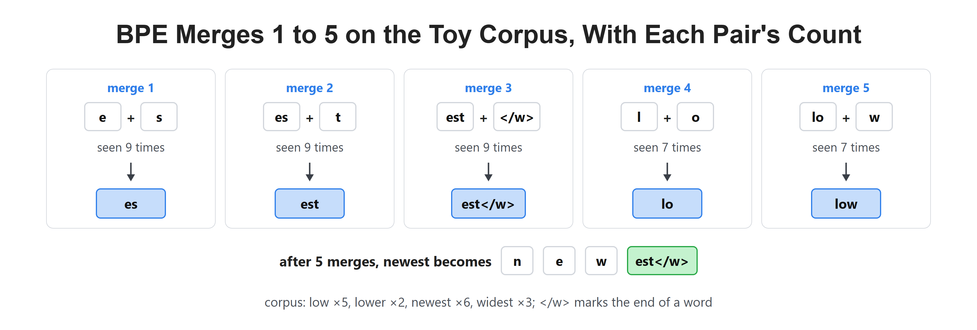
'newest' now tokenizes as: ('n', 'e', 'w', 'est</w>')Here, we can see BPE learn real shortcuts. The pair e and s is the most common, so it becomes es. Then es grows into est, and l and o grow into low. The </w> marker just means "end of word." After five merges, newest is not four letters and a suffix anymore. It reuses the est</w> piece it just learned. That reuse is the whole point: the model shares pieces across many words.
What About WordPiece and SentencePiece?
BPE has two close cousins that you will meet all the time.
WordPiece is what BERT uses. It works almost like BPE, but instead of merging the most frequent pair, it merges the pair that helps the model predict the text best. It marks the inside pieces of a word with ##, so playing becomes play and ##ing. That ## is just a flag that says "this piece joins the one before it."
SentencePiece takes a different view. It treats the whole text as one raw stream, spaces included, and marks a space with the symbol ▁. Because it does not need the text to be split into words first, it works cleanly for languages that do not use spaces, like Japanese, and for code. This makes it a strong choice for multilingual models.
Seeing Subwords in Real Code
Enough theory. Let's train a small BPE tokenizer with the Hugging Face tokenizers library and watch it split real words. We train it on a tiny word list, so it only knows a few pieces:
from tokenizers import Tokenizer
from tokenizers.models import BPE
from tokenizers.trainers import BpeTrainer
from tokenizers.pre_tokenizers import Whitespace

corpus = ["low", "lower", "lowest", "newer", "newest", "wider", "widest"]

tokenizer = Tokenizer(BPE(unk_token="[UNK]"))
tokenizer.pre_tokenizer = Whitespace()
trainer = BpeTrainer(vocab_size=50, special_tokens=["[UNK]"])
tokenizer.train_from_iterator([" ".join(corpus)] * 100, trainer)

for word in ["lowest", "slowest", "coldest"]:
    enc = tokenizer.encode(word)
print(f"{word!r:10} -> tokens {enc.tokens} ids {enc.ids}")'lowest' -> tokens ['lowest'] ids [26]
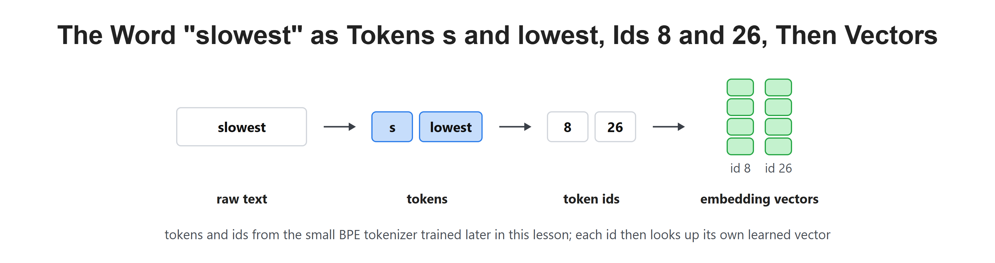
'slowest' -> tokens ['s', 'lowest'] ids [8, 26]
'coldest' -> tokens ['[UNK]', 'o', 'l', 'de', 'st'] ids [0, 6, 4, 14, 13]Here, we can see the three cases that matter. The word lowest was in the training text, so it stays as one whole token. The word slowest is new, but the tokenizer knows lowest, so it splits into s and lowest. And coldest uses letters the tokenizer barely saw, so it falls back to tiny pieces and even an [UNK] token for the part it cannot handle. This is why subword tokenizers rarely get truly stuck. When they meet a new word, they just use smaller pieces.
This also shows the trade-off at the heart of tokenization. A bigger vocabulary keeps more words whole, which makes each sentence shorter, but it costs more memory. A smaller vocabulary uses less memory, but it chops words into more pieces, which makes each sentence longer and slower. The [UNK] fallback, the byte-level safety net, and the special tokens like [UNK] are all there to make sure no input ever breaks the model. The number of tokens a model can read at once is called its context window, so shorter token lists also mean we can fit more text in.
From Tokens to Vectors: What Is an Embedding?
We now have token ids, but an id is just a name. The id 26 does not mean anything on its own, and id 27 is not "one more" than it in any useful way. We need to give each token a real meaning the model can compute with.
So, here comes the embedding to the rescue. An embedding is a list of numbers, a vector, attached to each token. In simple words, the model keeps a big table with one vector per token, and it looks up the vector for each id. During training, it slowly moves these vectors so that tokens with similar meaning end up close together.
Think of it like a map. Cities that are close in real life sit close on the map. In embedding space, words that are close in meaning, like king and queen, sit close together. The number of values in each vector is called the embedding dimension.
Let's look up a few embeddings with a small table:
import numpy as np
np.random.seed(42)

vocab_size, embed_dim = 10, 4
embedding_matrix = np.random.randn(vocab_size, embed_dim)  # the lookup table

token_ids = [7, 2, 5]
vectors = embedding_matrix[token_ids]

print("embedding_matrix shape:", embedding_matrix.shape)
print("token_ids:", token_ids)
print("looked-up vectors shape:", vectors.shape)
print("vector for token id 7:\n", vectors[0].round(3))embedding_matrix shape: (10, 4)
token_ids: [7, 2, 5]
looked-up vectors shape: (3, 4)
vector for token id 7:
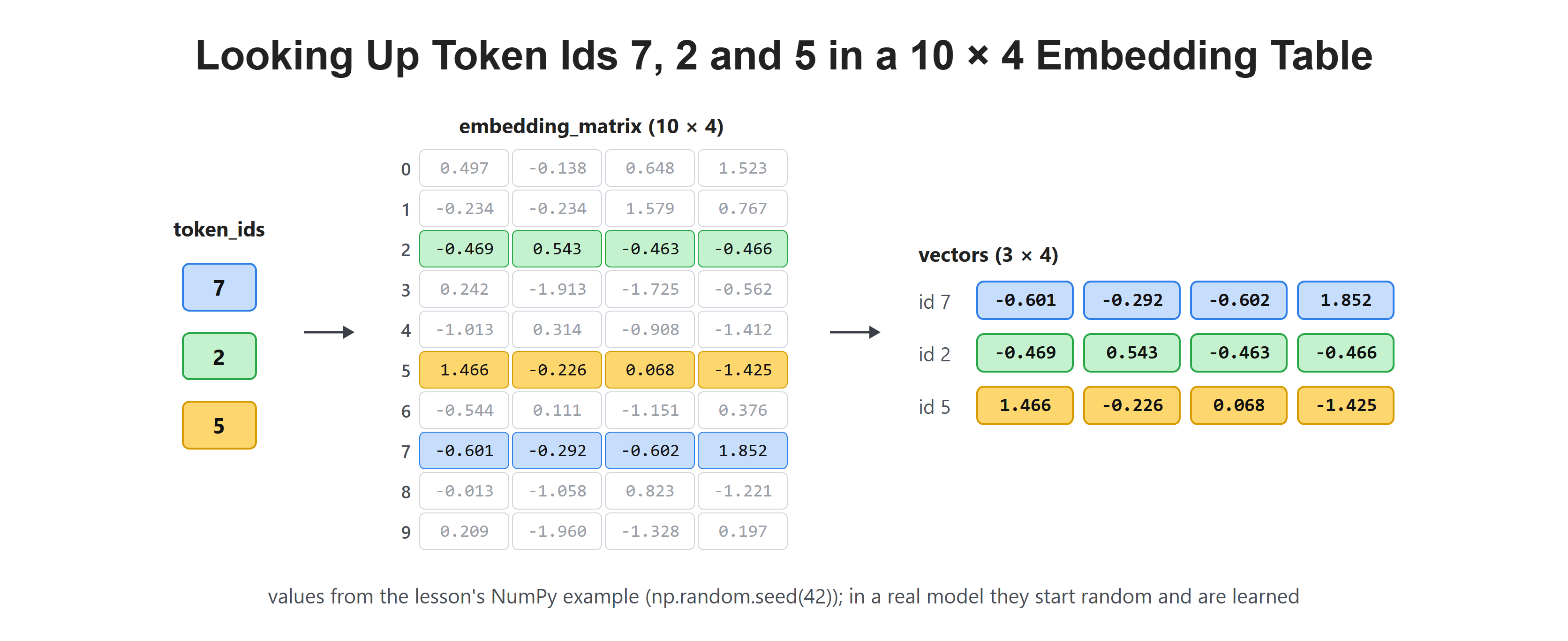
[-0.601 -0.292 -0.602 1.852]Here, we can see the whole idea in the shapes. Our table has 10 rows, one per token in the vocabulary, and 4 numbers per row. We asked for three token ids, so we got back three vectors, each with four numbers. In a real model these vectors have hundreds or thousands of numbers, and they start random but learn meaning during training.
Why Do We Need Attention?
Our sentence is now a list of vectors, one per token. But there is still a problem. Each vector only knows about its own token. Read this sentence: "The trophy did not fit in the suitcase because it was too big." What does "it" mean, the trophy or the suitcase? To answer, a word must be able to look at the other words around it.
So, here comes attention to the rescue. Attention is the mechanism that lets every token look at every other token and pull in the information it needs. It is the single most important idea in the Transformer.
Self-Attention: Query, Key, and Value
Self-attention gives each token three roles, and the names come from a library.
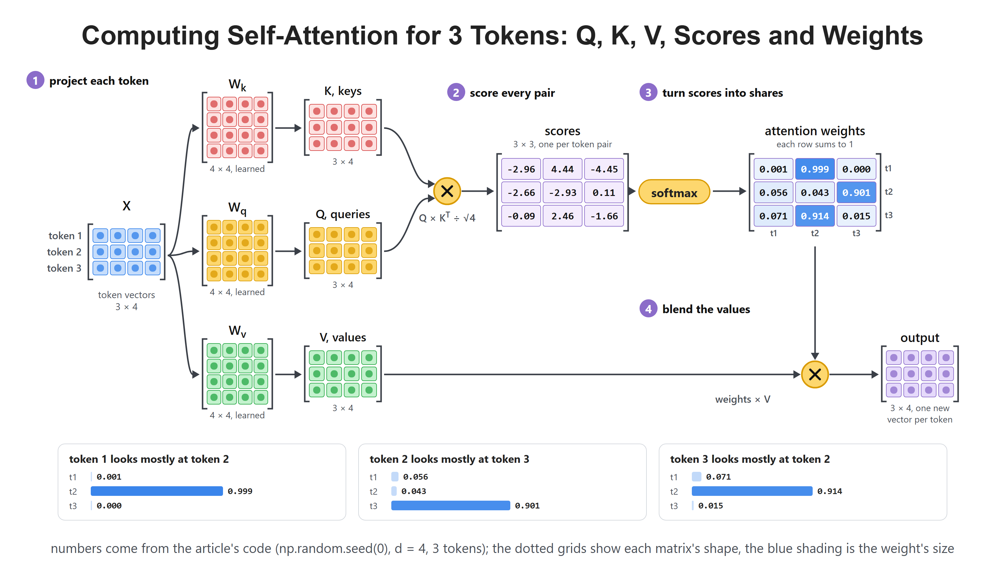
The query is what a token is looking for, like a search request. The key is a label on every other token, like the title on a book's spine. The value is the actual content each token carries, like the words inside the book. Each token compares its query against every key to see which tokens are relevant, and then it collects a blend of their values.
The strength of each match is called an attention weight. For each token, these weights add up to 1, so they act like shares of attention split across the sentence. Let's compute them for three tokens:
import numpy as np
np.random.seed(0)

d = 4
X = np.random.randn(3, d)  # 3 token vectors

W_q, W_k, W_v = np.random.randn(d, d), np.random.randn(d, d), np.random.randn(d, d)
Q, K, V = X @ W_q, X @ W_k, X @ W_v   # queries, keys, values

scores = Q @ K.T / np.sqrt(d)         # how well each query matches each key

def softmax(z):
    e = np.exp(z - z.max(axis=-1, keepdims=True))
    return e / e.sum(axis=-1, keepdims=True)

weights = softmax(scores)             # turn scores into shares that sum to 1
output = weights @ V                  # blend the values

print("attention weights (each row sums to 1):")
print(weights.round(3))
print("row sums:", weights.sum(axis=1).round(3))
print("output shape:", output.shape)attention weights (each row sums to 1):
[[0.001 0.999 0. ]
[0.056 0.043 0.901]
[0.071 0.914 0.015]]
row sums: [1. 1. 1.]Here, we can see attention in action. Each row is one token deciding how much to look at the others. The first token puts almost all of its attention (0.999) on the second token. The second token looks mostly at the third. Every row sums to 1, so each token spends exactly one full unit of attention, split across the sentence. The output blends the values using these shares, so every token walks away richer, carrying a little of what it needed from the others.
Multi-Head Attention
One round of attention learns one kind of relationship. But language has many at once. One head might track which word is the subject, another might track tense, another might link a pronoun to its noun.
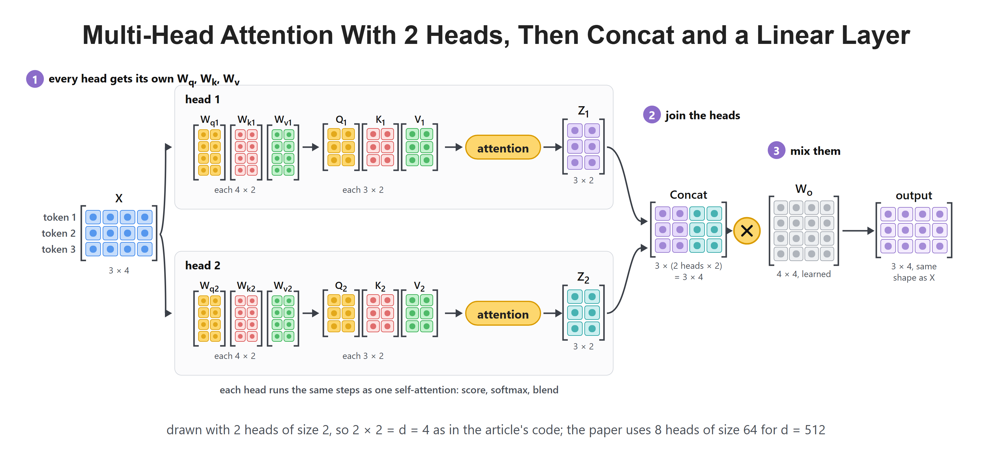
So instead of running attention once, we run it several times in parallel. Each copy is called a head, and each head learns to look for a different kind of link. We then join their results back together. This is multi-head attention, and it is why a Transformer can follow grammar, meaning, and long-range links all at the same time.
Think of it like several readers going through the same page. One reads for the plot, one for the names, one for the dates. Together they understand far more than any single reader could.
Masked (Causal) Attention
There is one case where a token must not see everything. When a model writes text one word at a time, it must not peek at the words that come later, because during real use those words do not exist yet.
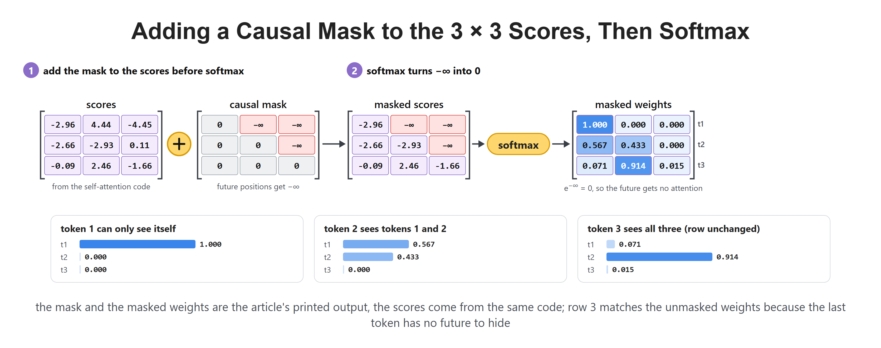
So we block the future with a causal mask. Before we turn the scores into weights, we set every "future" position to negative infinity. After the softmax, those spots become exactly zero, so a token can only attend to itself and the tokens before it. This is what makes generation honest.
mask = np.triu(np.ones((3, 3)) * -np.inf, k=1)   # block the upper triangle
print("causal mask (upper triangle blocked):")
print(mask)

masked = softmax(scores + mask)
print("masked attention weights:")
print(masked.round(3))causal mask (upper triangle blocked):
[[ 0. -inf -inf]
[ 0. 0. -inf]
[ 0. 0. 0.]]
masked attention weights:
[[1. 0. 0. ]
[0.567 0.433 0. ]
[0.071 0.914 0.015]]Here, we can see the effect clearly. The first token can only look at itself, so its weight is 1.0 and the rest are 0. The second token can look at the first two but not the third. Only the last token can see everything. The staircase of zeros in the top-right corner is the future being hidden.
Positional Encoding
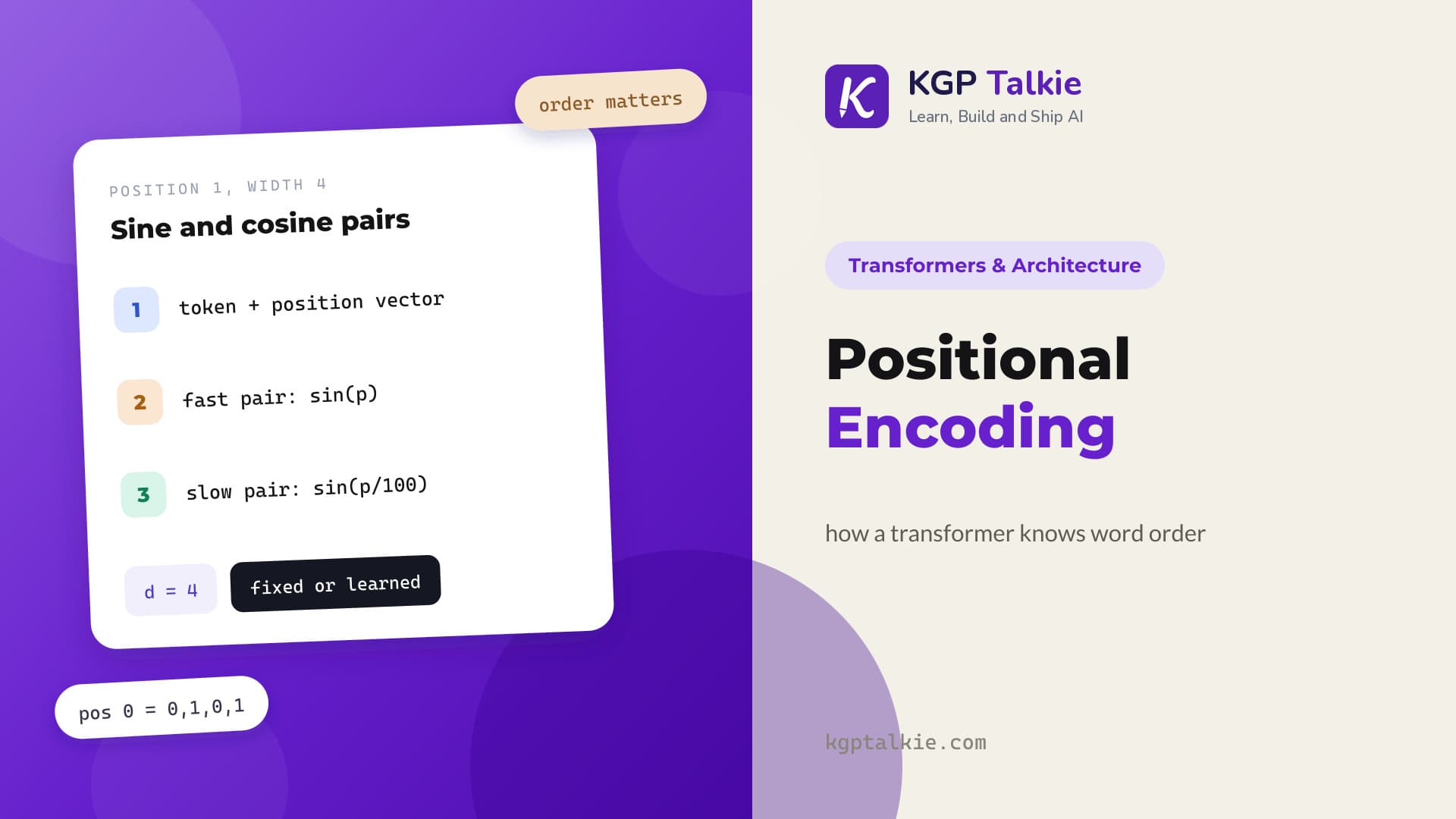
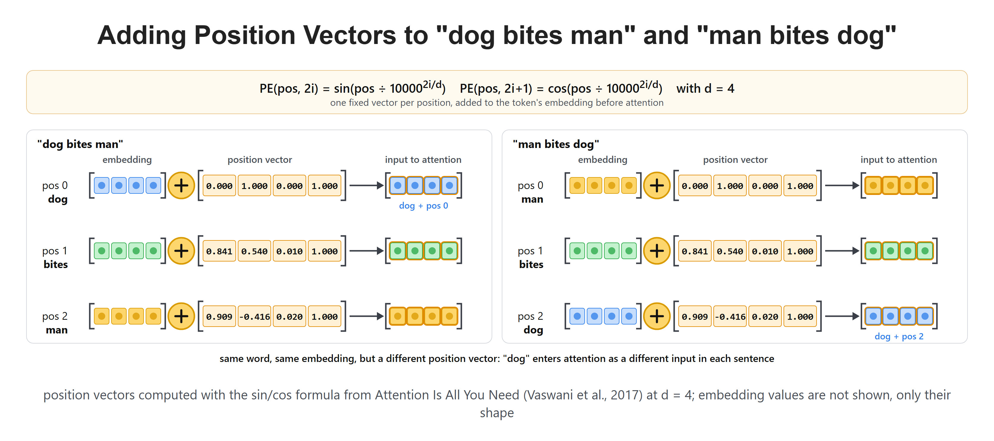
Attention has a hidden weakness. On its own, it treats a sentence like a bag of words with no order. Shuffle the words and the raw attention math gives the same answer. But "dog bites man" and "man bites dog" are very different, so order clearly matters.
So we add order back in with positional encoding. Before attention runs, we add a small position signal to each token's embedding, one unique pattern for position 1, another for position 2, and so on. Now every vector carries both its meaning and its place in the line, and attention can tell first from last.
Cross-Attention
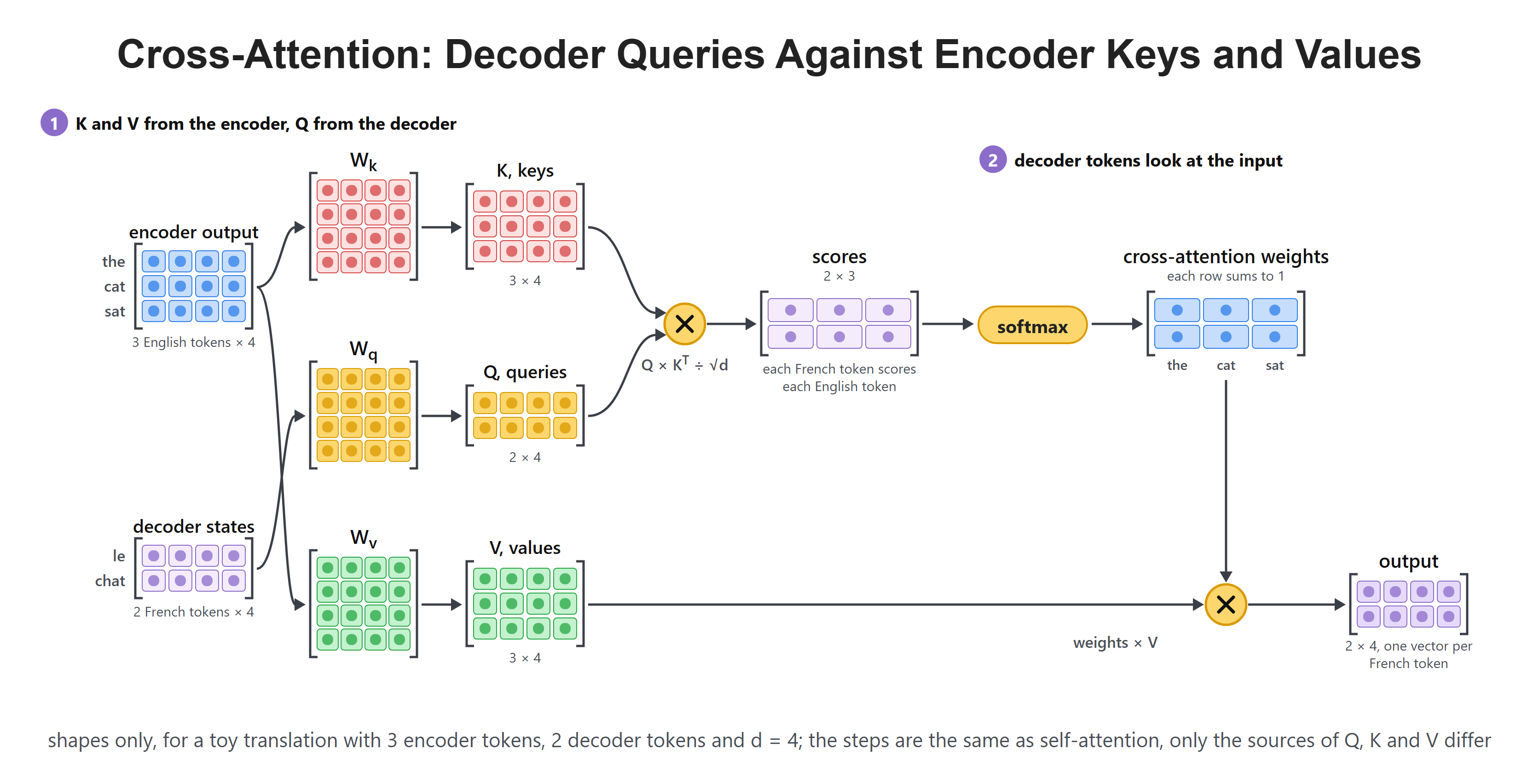
So far every token has looked at tokens in the same sentence. Cross-attention is the version where one sequence looks at a different one. It is the bridge used when a model reads one input and writes a separate output, like translating English into French. The queries come from the output side, while the keys and values come from the input side. This lets the words being generated look back at the full input and stay faithful to it. We will see exactly where this fits in the next section.
The Three Families of Transformers
Every Transformer is built from the pieces we just met, but they are wired in three different ways. Each wiring suits a different kind of task.
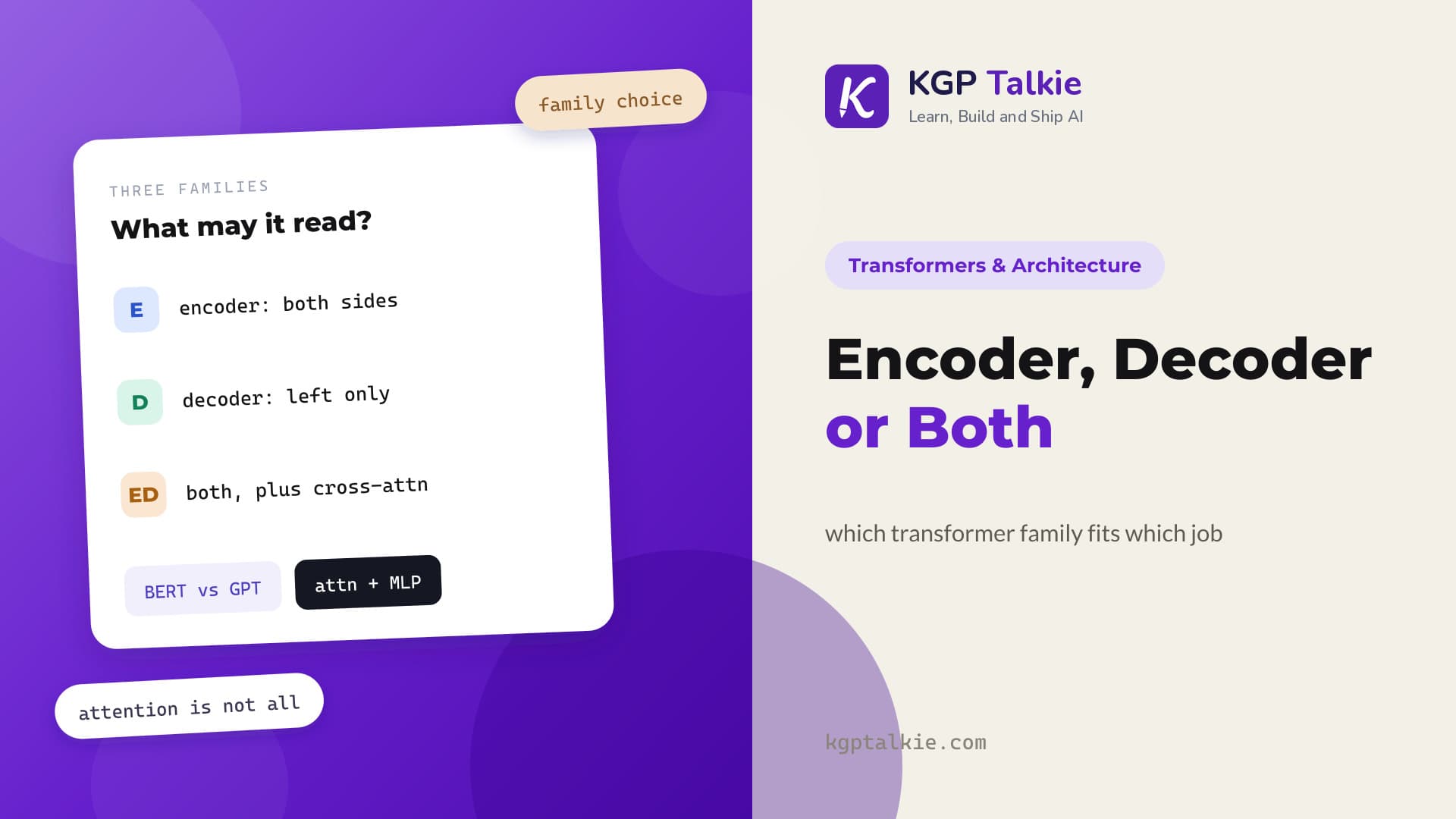
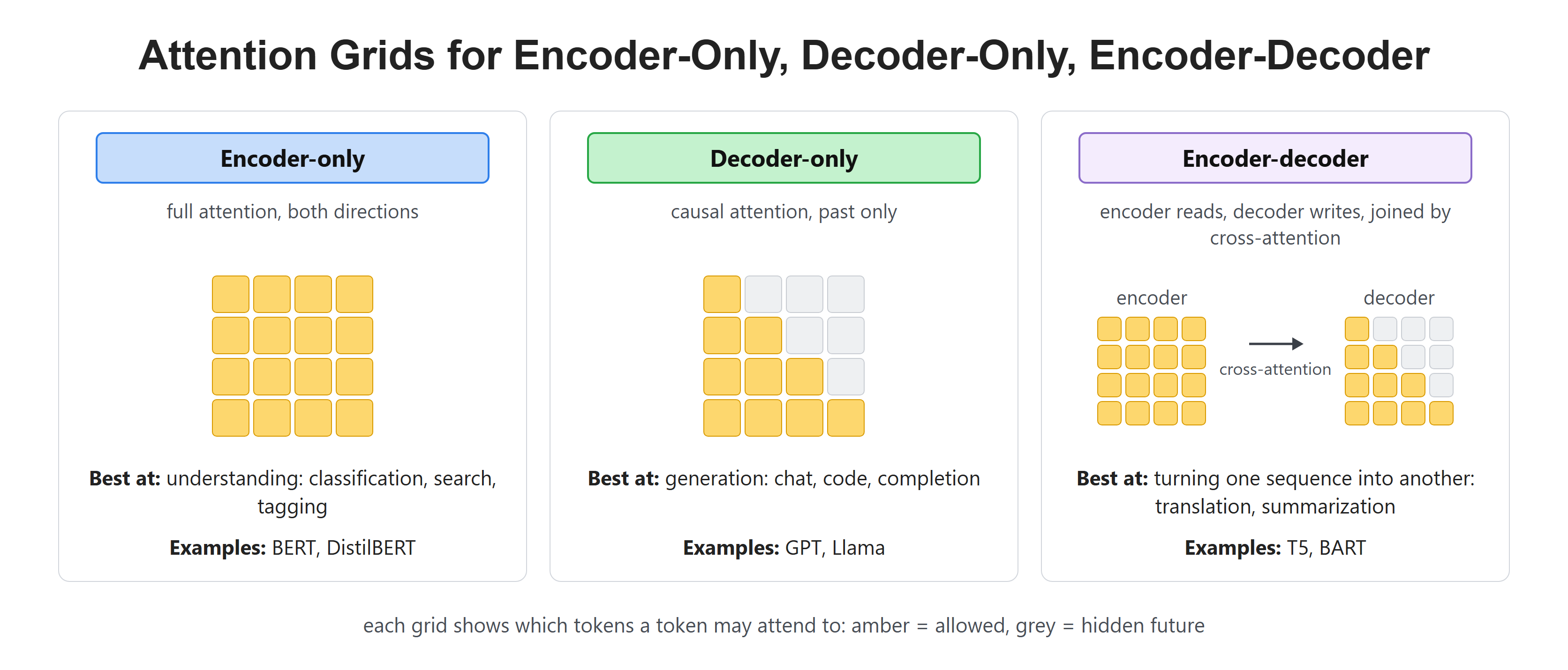
An encoder-only Transformer, like BERT, reads the whole input at once and lets every token see every other token in both directions. Because it sees the full sentence, it is great at understanding tasks: classification, search, and picking out names. It reads, but it does not generate.
A decoder-only Transformer, like GPT, is the opposite. It uses the causal mask so each token sees only the past, and it writes text one token at a time. This is the family behind chatbots and code assistants. It generates.
An encoder-decoder Transformer, like T5, uses both. The encoder reads the input in full, and the decoder writes the output one token at a time. The two are joined by cross-attention, so every word being written can look back at the whole input. This suits tasks that turn one sequence into another, like translation and summarization.
Let me tabulate the three families for your better understanding.
| Family | Attention style | Best at | Examples |
|---|---|---|---|
| Encoder-only | Full, both directions | Understanding: classification, search, tagging | BERT, DistilBERT |
| Decoder-only | Causal, past only | Generation: chat, code, completion | GPT, Llama |
| Encoder-decoder | Encoder reads, decoder writes, joined by cross-attention | Turning one sequence into another: translation, summarization | T5, BART |
Inside a Decoder-Only Model: GPT-2
Let's put every piece from this lesson together inside one real decoder-only model: GPT-2 small, with 124M parameters. At the bottom, each token id picks its row from a token embedding table of 50,257 × 768. GPT-2 then adds a position vector to each one. These position vectors do not come from a fixed formula. GPT-2 learns them in training, one for each of its 1,024 positions.
Then the vectors pass through 12 identical Transformer blocks, one after another. Each block does two jobs. First, masked multi-head attention lets every token look back at itself and the tokens before it, using 12 heads of 64 numbers each. Then a small MLP widens each vector from 768 to 3,072 numbers and shrinks it back to 768. A LayerNorm runs before each job, and a residual connection adds the job's input back to its output.
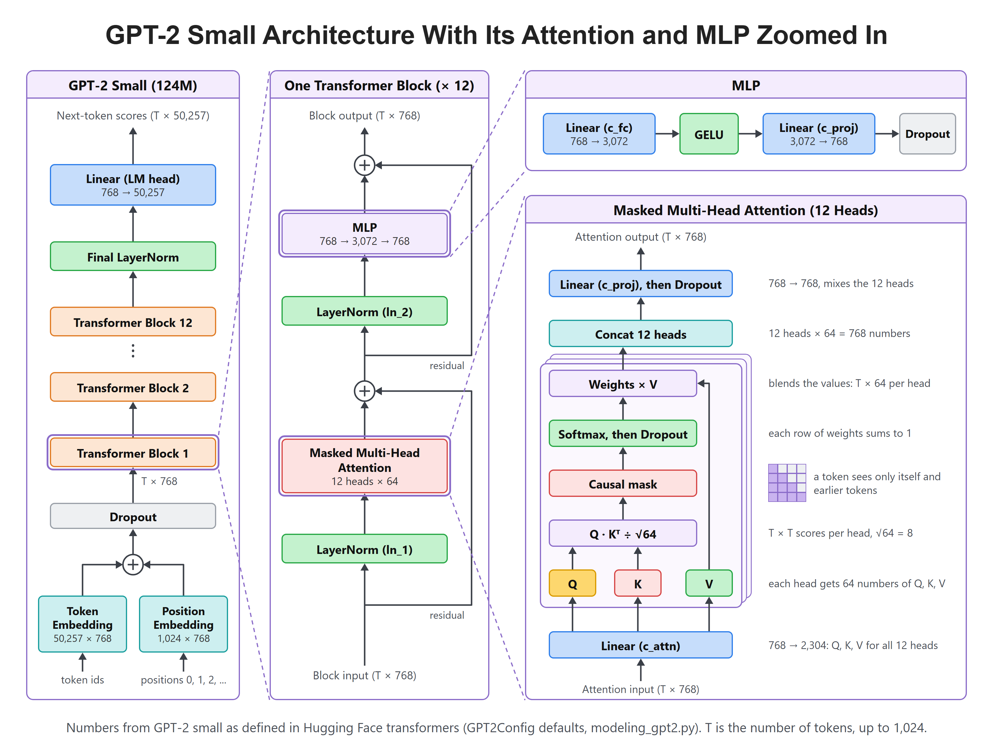
Here, we can see the whole model on the left, one block in the middle, and the attention and MLP zoomed in on the right. After the last block, one more LayerNorm and a final Linear layer turn each 768-number vector into 50,257 scores, one for every token in the vocabulary. The highest score at the last position tells us which token is most likely to come next.
Recap
This is how a Transformer reads text. We started with raw text and chopped it into tokens using subword methods like BPE, WordPiece, and SentencePiece, so no new word ever breaks the model. We turned those token ids into embeddings, points in a space where meaning lives. Attention then let every token look at every other token, multi-head attention gave it several views at once, and the causal mask kept generation honest by hiding the future. Positional encoding put word order back in. Finally, we met the three families: encoder-only for understanding, decoder-only for generation, and encoder-decoder for turning one sequence into another.
In the next module, we roll up our sleeves and fine-tune all three families on our own data. That is Module 02: Hands-On Fine-Tuning of Transformers, coming next in this series.