
Word Embedding and Sentiment Analysis
In this blog, we will learn how to build a word embedding model for Twitter sentiment analysis with TensorFlow and Keras. We take raw tweets, turn them into number sequences, and train a small CNN to tell a positive tweet from a negative one. In simple words, the model learns which words carry a good feeling and which carry a bad one.
What is Word Embedding?
Natural Language Processing (NLP) refers to computer systems designed to understand human language. Human language, like English or Hindi, consists of words and sentences, and NLP attempts to extract information from these sentences.
Machine learning and deep learning algorithms only take numeric input, so how do we convert text to numbers?
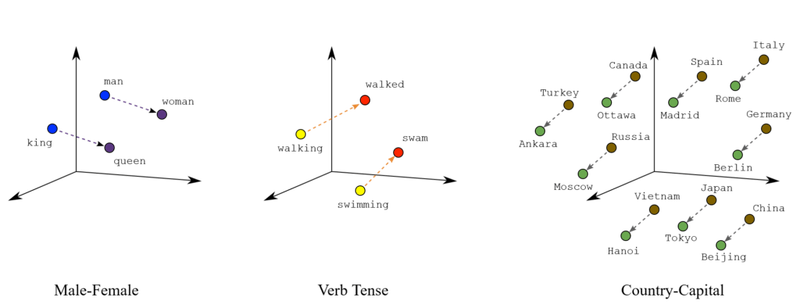
A word embedding is a learned representation for text where words that have the same meaning have a similar representation. Embeddings translate large sparse vectors into a lower-dimensional space that preserves semantic relationships. Word embeddings represent individual words as real-valued vectors in a lower-dimensional space. The sparse matrix problem with BOW is solved by mapping high-dimensional data into a lower-dimensional space. The lack of meaningful relationship in BOW is solved by placing vectors of semantically similar items close to each other. This way, words with similar meaning have similar distances in the vector space, as shown below. "king is to queen as man is to woman" is encoded in the vector space, and verb tense along with country/capital pairs are also encoded in low-dimensional space, preserving the semantic relationships.
Dataset
Sentiment140 Dataset on Kaggle
This is the Sentiment140 dataset. It contains 1,600,000 tweets extracted using the Twitter API.
We are going to use 4,000 tweets to train our model. The tweets have been annotated (0 = negative, 1 = positive) and can be used to detect sentiment.
You can download the modified dataset from here.
Watch Full Video:
The imports below bring in everything needed for this tutorial.
pandasis used to read the dataset.numpyis used to perform basic array operations.Tokenizeris used to split the text into tokens.pad_sequencesis used to pad the data if necessary.train_test_splitfromsklearnis used split the data into training and testing dataset.- The other components are imported to build the neural network.
from tensorflow.keras.preprocessing.text import Tokenizer
from tensorflow.keras.preprocessing.sequence import pad_sequences
from tensorflow.keras.models import Sequential
from tensorflow.keras.layers import Dense,Flatten,Embedding,Activation, Dropout
from tensorflow.keras.layers import Conv1D, MaxPooling1D, GlobalMaxPooling1D
import numpy as np
from numpy import array
import pandas as pd
from sklearn.model_selection import train_test_split
read_csv loads the data into the dataframe. data.head() shows the first 5 rows of the dataset.
df = pd.read_csv('twitter4000.csv')
df.head()| twitts | sentiment | |
|---|---|---|
| 0 | is bored and wants to watch a movie any sugge... | 0 |
| 1 | back in miami. waiting to unboard ship | 0 |
| 2 | @misskpey awwww dnt dis brng bak memoriessss, ... | 0 |
| 3 | ughhh i am so tired blahhhhhhhhh | 0 |
| 4 | @mandagoforth me bad! It's funny though. Zacha... | 0 |
The value_counts() function shows the distribution of sentiment in the dataset. There are 2,000 positive sentiment reviews and 2,000 negative reviews.
df['sentiment'].value_counts()1 2000
0 2000
Name: sentiment, dtype: int64Get the tweet text as a list.
text = df['twitts'].tolist()
text[:10]['is bored and wants to watch a movie any suggestions?', 'back in miami. waiting to unboard ship ', "@misskpey awwww dnt dis brng bak memoriessss, I thnk I'm sad. LoL", 'ughhh i am so tired blahhhhhhhhh', "@mandagoforth me bad! It's funny though. Zachary Quinto is only there for a few though. & to reply just put the @ symbol before the name!", "brr, i'm so cold. at the moment doing my assignment on Huntington's Disease, which is really depressing ", "@kevinmarquis haha yep but i really need to sleep, i feel like crap lol cant sleep when he's away god i'm pathetic!", "eating some ice-cream while I try to see @peterfacinelli's followers numbre raise...not working sadly ", '@phatty84 just hella bored at work lol', 'Food poisoning blowssss ']Get the labels in y.
y = df['sentiment']The Tokenizer() class converts text to numbers. It vectorizes a text corpus by turning each text into either a sequence of integers (each integer being the index of a token in a dictionary) or into a vector where the coefficient for each token could be binary, based on word count, or based on tf-idf.
token = Tokenizer()
token.fit_on_texts(text)
token
word_index is an index to word dictionary so every word gets a unique integer value. It starts from 0, so we add 1 to get the vocab_size. vocab_size is the total number of unique words in the dataset.
vocab_size = len(token.word_index) + 1
vocab_size10135index_word is the index to word dictionary. The first 100 key-value pairs of the dictionary look like this.
import itertools
print(dict(itertools.islice(token.index_word.items(), 100))){1: 'i', 2: 'to', 3: 'the', 4: 'a', 5: 'my', 6: 'and', 7: 'you', 8: 'is', 9: 'it', 10: 'in', 11: 'for', 12: 'of', 13: 'me', 14: 'on', 15: 'so', 16: 'that', 17: "i'm", 18: 'have', 19: 'at', 20: 'but', 21: 'just', 22: 'was', 23: 'with', 24: 'not', 25: 'be', 26: 'this', 27: 'day', 28: 'up', 29: 'now', 30: 'good', 31: 'all', 32: 'get', 33: 'out', 34: 'go', 35: 'no', 36: 'http', 37: 'today', 38: 'like', 39: 'are', 40: 'love', 41: 'your', 42: 'quot', 43: 'too', 44: 'lol', 45: 'work', 46: 'got', 47: "it's", 48: 'amp', 49: 'do', 50: 'com', 51: 'u', 52: 'back', 53: 'going', 54: 'what', 55: 'time', 56: 'from', 57: 'had', 58: 'will', 59: 'know', 60: 'about', 61: 'im', 62: 'am', 63: "don't", 64: 'can', 65: 'one', 66: 'really', 67: "can't", 68: 'we', 69: 'oh', 70: 'well', 71: 'still', 72: '2', 73: 'some', 74: 'its', 75: 'miss', 76: 'want', 77: 'see', 78: 'when', 79: 'home', 80: 'think', 81: 'an', 82: 'as', 83: 'if', 84: 'night', 85: 'need', 86: 'again', 87: 'new', 88: 'there', 89: 'morning', 90: 'here', 91: 'how', 92: 'her', 93: 'much', 94: 'thanks', 95: 'or', 96: 'they', 97: '3', 98: 'last', 99: 'off', 100: 'more'}If x = 'i to the a and' is the input text, the tokenizer encodes it as shown below.
x = ['i to the a and']
token.texts_to_sequences(x)[[1, 2, 3, 4, 6]]Encode text, which contains all the tweets.
encoded_text = token.texts_to_sequences(text)
print(encoded_text[:30])[[8, 304, 6, 345, 2, 191, 4, 236, 254, 3079], [52, 10, 1019, 206, 2, 3080, 3081], [3082, 1197, 668, 1955, 3083, 1956, 3084, 1, 3085, 17, 115, 44], [1957, 1, 62, 15, 192, 3086], [3087, 13, 113, 47, 328, 136, 3088, 3089, 8, 101, 88, 11, 4, 285, 136, 48, 2, 448, 21, 277, 3, 3090, 218, 3, 449], [3091, 17, 15, 315, 19, 3, 892, 164, 5, 1459, 14, 3092, 3093, 386, 8, 66, 1460], [3094, 110, 366, 20, 1, 66, 85, 2, 108, 1, 117, 38, 536, 44, 182, 108, 78, 346, 207, 305, 17, 3095], [450, 73, 537, 569, 295, 1, 316, 2, 77, 3096, 367, 3097, 1461, 24, 187, 893], [3098, 21, 1958, 304, 19, 45, 44], [409, 3099, 3100], [3101, 132, 609, 79, 3, 193, 368, 17, 131, 3, 158, 199], [3102, 127, 1, 139, 226, 2, 1020, 9, 29, 1, 222, 74, 55, 2, 3103, 16, 3104], [67, 894, 423], [1959, 119, 52, 56, 211, 159, 387, 669, 48, 68, 255, 1462, 3, 3105, 71, 570, 5, 1959, 329], [1960, 3106, 3107, 46, 3108, 3109], [3110, 1463, 70, 19, 227, 17, 28, 2], [3111, 1, 245, 212, 1961, 51, 72, 36, 146, 246, 3112, 1, 538, 20, 74, 507, 1962, 410, 1, 1198, 219, 787], [3113, 69, 1, 1021, 5, 3114, 33, 2, 1199, 451, 263, 12, 9, 388, 1, 143, 76, 2, 316, 1464, 73, 159, 1465], [3115, 3116, 31, 12, 39, 3117, 9, 20, 96, 39, 24, 1466, 3118, 1200, 386, 507, 369, 15, 68, 571, 32, 2, 1022, 2, 51], [3119, 165, 88, 35, 64, 49, 1963, 6, 24, 52, 10, 572, 306, 1467, 176, 152, 75, 7], [3120, 15, 788, 78, 9, 610, 95, 91, 20, 1, 3121, 789, 370, 7, 91, 39, 7, 91, 18, 7, 102], [54, 8, 28, 23, 5, 3122], [52, 3123, 86, 37, 611, 15, 473, 452, 82, 1201, 101, 719, 153, 1468, 790, 11, 188, 3124], [3125, 69, 1, 670, 83, 3, 1964, 14, 3, 1469, 8, 720, 2, 34], [3126, 7, 347, 42, 3127, 11, 573, 42, 1, 22, 1965, 1966], [3128, 87, 671, 8, 101, 3129, 153, 207, 256, 16, 8, 1023], [1470, 3, 3130, 38, 35, 223], [539, 1, 18, 4, 389, 10, 5, 1967, 43], [1, 612, 2, 18, 255, 5, 1024, 1471], [52, 56, 3, 424, 3131, 102, 4, 148, 55, 508, 1, 98, 57, 3132, 3133, 3134, 3135, 227, 3136, 8, 14, 92, 116, 2, 791, 13]]Each tweet has a different length. All encoded tweets must have the same length before going into the neural network. pad_sequences pads zeros to tweets shorter than 120 tokens.
max_length = 120
X = pad_sequences(encoded_text, maxlen=max_length, padding='post')
print(X)[[ 8 304 6 ... 0 0 0]
[ 52 10 1019 ... 0 0 0]
[ 3082 1197 668 ... 0 0 0]
...
[ 1033 21 1021 ... 0 0 0]
[10134 134 7 ... 0 0 0]
[ 94 11 226 ... 0 0 0]]All 4,000 tweets now have the same length of 120.
X.shape(4000, 120)Split the data into training and test sets using train_test_split(). 80% goes to training and 20% to testing. random_state controls the shuffling before the split. stratify = y splits the data in a stratified fashion using y as the class labels.
X_train, X_test, y_train, y_test = train_test_split(X, y, random_state = 42, test_size = 0.2, stratify = y)A Sequential() model is appropriate for a plain stack of layers where each layer has exactly one input tensor and one output tensor.
The Embedding() layer is initialized with random weights and will learn an embedding for all of the words in the training dataset.
It requires 3 arguments:
input_dim: The size of the vocabulary in the text data, which is 10,135 in our case.output_dim: The size of the vector space in which words will be embedded. It defines the size of the output vectors from this layer for each word. We have set it to 300.input_length: Length of input sequences when it is constant. In our case it is 120.
Conv1D() is a 1D Convolution Layer. This layer works well for extracting features from a fixed-length segment of the overall dataset when the location of the feature within the segment is not the main concern. In the Conv1D() layer we learn a total of 64 filters with a convolutional window size of 8, using the ReLU activation function. The rectified linear activation function, ReLU, is a piecewise linear function that outputs the input directly if it is positive, otherwise it outputs zero.
MaxPool1D() downsamples the input representation by taking the maximum value over the window defined by pool_size, which is 2 in this neural network.
Dropout() randomly sets the outgoing edges of hidden units to 0 at each update of the training phase. The value passed in dropout specifies the probability at which outputs of the layer are dropped out.
GlobalMaxPooling1D() downsamples the input representation by taking the maximum value over the time dimension.
Dense() is the regular deeply connected neural network layer. The output layer is a dense layer with 1 neuron because we are predicting a single value. The Sigmoid function is used because it outputs values between 0 and 1, which works for binary prediction.
vec_size = 300

model = Sequential()
model.add(Embedding(vocab_size, vec_size, input_length=max_length))

model.add(Conv1D(64, 8, activation = 'relu'))
model.add(MaxPooling1D(2))
model.add(Dropout(0.2))

model.add(Dense(32, activation='relu'))
model.add(Dropout(0.5))

model.add(Dense(16, activation='relu'))

model.add(GlobalMaxPooling1D())

model.add(Dense(1, activation='sigmoid'))
Compile the model and fit it to the training data. Training runs for 5 epochs. An epoch is one full pass over the training data. validation_data is the data used to evaluate loss and metrics at the end of each epoch; the model does not train on it. Setting metrics = ['accuracy'] tells the model to track accuracy.
model.compile(optimizer='adam', loss = 'binary_crossentropy', metrics = ['accuracy'])%%time
model.fit(X_train, y_train, epochs = 5, validation_data = (X_test, y_test))Train on 3200 samples, validate on 800 samples
Epoch 1/5
3200/3200 [==============================] - 8s 2ms/sample - loss: 0.6937 - acc: 0.4919 - val_loss: 0.6870 - val_acc: 0.5188
Epoch 2/5
3200/3200 [==============================] - 6s 2ms/sample - loss: 0.6588 - acc: 0.6212 - val_loss: 0.6328 - val_acc: 0.6425
Epoch 3/5
3200/3200 [==============================] - 5s 2ms/sample - loss: 0.5100 - acc: 0.7625 - val_loss: 0.6255 - val_acc: 0.6787
Epoch 4/5
3200/3200 [==============================] - 6s 2ms/sample - loss: 0.3110 - acc: 0.8763 - val_loss: 0.7330 - val_acc: 0.6925
Epoch 5/5
3200/3200 [==============================] - 6s 2ms/sample - loss: 0.1663 - acc: 0.9394 - val_loss: 0.7949 - val_acc: 0.6775
Wall time: 33.8 sTest the model by predicting sentiments on unseen tweets. The get_encoded() function pre-processes new text the same way as the training data. predict_classes() returns the predicted class label.
def get_encoded(x):
    x = token.texts_to_sequences(x)
    x = pad_sequences(x, maxlen=max_length, padding = 'post')
    return x

x = ['worst services. will not come again']
model.predict_classes(get_encoded(x))array([[0]])x = ['thank you for watching']
model.predict_classes(get_encoded(x))array([[1]])Training on the full 1,600,000-tweet dataset would improve accuracy further. Adding preprocessing steps like spelling correction and repeated-letter normalization would also help.
Conclusion
In this blog, we built a CNN text classifier using a trainable word embedding layer on the Sentiment140 Twitter dataset. Starting from raw tweet text, we tokenized and padded 4,000 tweets into fixed-length integer sequences, trained an Embedding layer alongside a Conv1D architecture, and reached 69% validation accuracy in 5 epochs on an 80/20 split.
Key takeaways:
- Word embeddings solve the sparsity problem of Bag-of-Words by mapping words to dense, low-dimensional vectors where semantically similar words cluster together. "king" and "queen" occupy nearby positions.
- Keras
Tokenizerconverts text to integer indices;pad_sequencesnormalizes sequence lengths to a fixedmaxlenby zero-padding short sequences at the end (padding='post'). Conv1Dtreats text as a 1D signal and learns local n-gram features;GlobalMaxPooling1Dcollapses the sequence dimension by taking the maximum activation across all positions.- 4,000 tweets is a small sample from Sentiment140's 1.6M. Training on the full dataset would substantially improve accuracy beyond the 69% shown here.
Next steps:
- Scale to the full 1.6M Sentiment140 dataset and add preprocessing (spelling correction, repeated-character normalization) to push accuracy above 80%.
- Replace the trainable Embedding layer with pre-trained GloVe vectors as in Words Embedding Using GloVe Vectors to compare transfer learning versus learning from scratch.
- Swap the Conv1D for an LSTM to capture long-range sequential dependencies in tweet text and compare validation accuracy on the same dataset.