What Are Embeddings? From Token IDs to Meaning

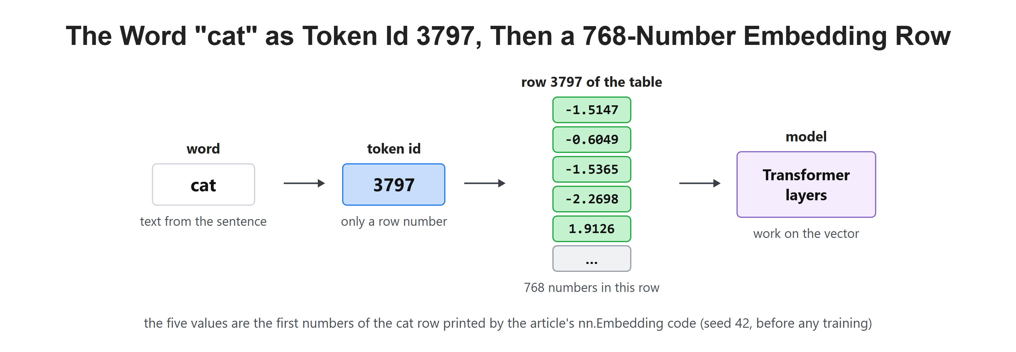
We spent nine days turning text into numbers. A sentence is now a list of token IDs like [464, 3797, 3332]. But those numbers are just row labels. Token 3797 is not bigger or better than token 464. It is simply row 3797 in a list.

So how does a model get from a row number to meaning? That is the job of embeddings, and it is the first real layer of every Transformer. In simple words, an embedding is a list of numbers that the model looks up for each token.

In this blog, we will learn why one-hot encoding fails, how the embedding table works, and how its numbers learn meaning during training.

A Token ID Is Just a Name Tag

Let's start with what an ID is not. It is not a measurement. If "cat" is 3797 and "dog" is 3798, those two are neighbours by an accident of how the vocabulary was built, not because they mean similar things.

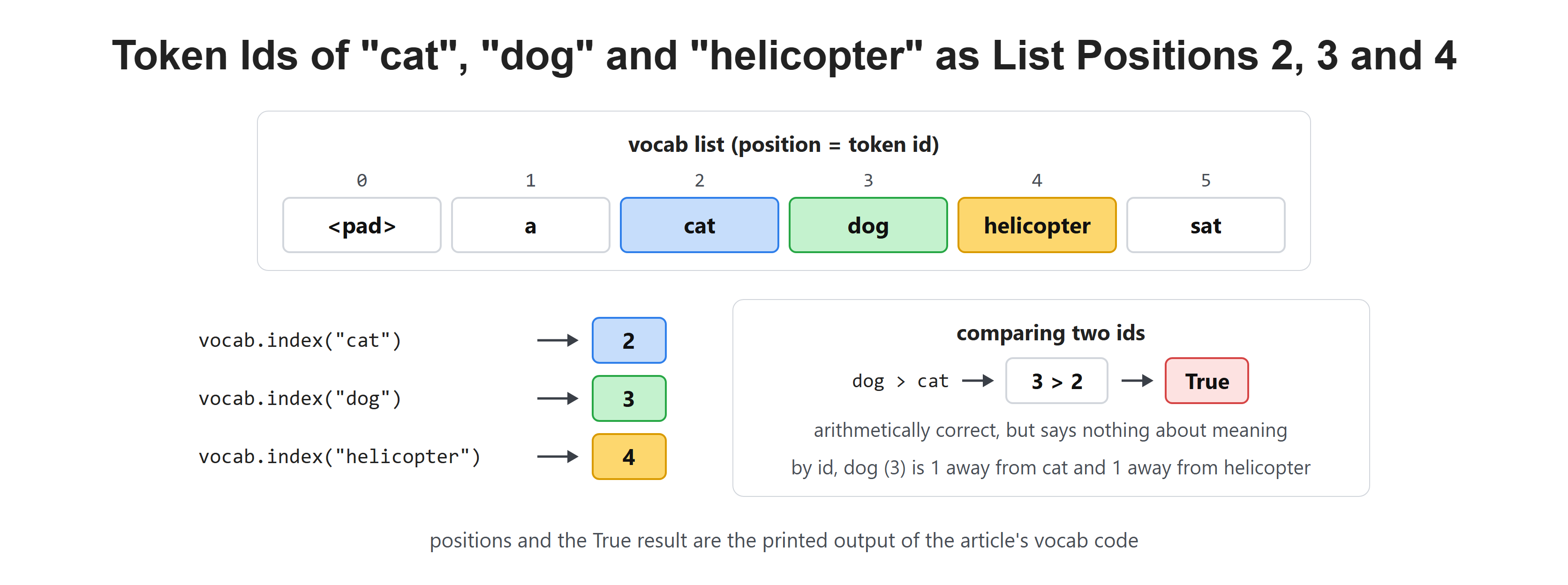
Now, we build a tiny vocabulary of our own and look at what an ID really is. This is a separate toy example, so "cat" gets a different ID here than the 3797 above. The vocabulary is just a list, and the ID is the position in that list.

vocab = ["<pad>", "a", "cat", "dog", "helicopter", "sat"]

print("cat        ->", vocab.index("cat"))
print("dog        ->", vocab.index("dog"))
print("helicopter ->", vocab.index("helicopter"))

# the id is only a position, so comparing ids says nothing about meaning
print("is dog 'more' than cat?", vocab.index("dog") > vocab.index("cat"))

cat        -> 2
dog        -> 3
helicopter -> 4
is dog 'more' than cat? True

That last line is the point. Python happily answers True, because 3 is greater than 2. The comparison is correct as math and means nothing at all. IDs are labels, not quantities. The number identifies a row and nothing more.

The Obvious Idea That Fails: One-Hot

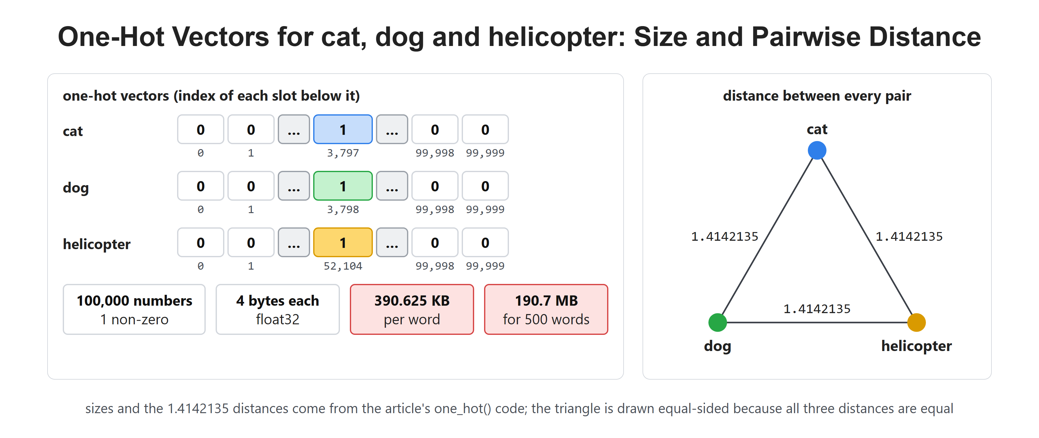
The first idea most people have is one-hot encoding. We give every token a long list of zeros with a single one in its own position.

It works, and it is easy to write. Let's measure what it costs:

import numpy as np

VOCAB_SIZE = 100_000

def one_hot(token_id):
    vec = np.zeros(VOCAB_SIZE, dtype=np.float32)
    vec[token_id] = 1.0
    return vec

cat = one_hot(3797)
print("numbers per word :", cat.size)
print("non-zero values  :", int(cat.sum()))
print("memory per word  :", cat.nbytes / 1024, "KB")

numbers per word : 100000
non-zero values  : 1
memory per word  : 390.625 KB

One hundred thousand numbers to store a single word, and 99,999 of them are zero. A 500-word paragraph would cost about 190 MB.

Waste is the smaller problem. The real failure is that one-hot cannot show that two words are related. When we measure the distance between three words, we get the same answer every time:

dog = one_hot(3798)
helicopter = one_hot(52104)

print("cat vs dog        :", np.linalg.norm(cat - dog))
print("cat vs helicopter :", np.linalg.norm(cat - helicopter))

cat vs dog        : 1.4142135
cat vs helicopter : 1.4142135

Identical, down to the last digit. In one-hot space, a cat is exactly as far from a dog as it is from a helicopter. Each word has its own private column, and no two words ever share anything. The format has no way to say "these two are similar".

The Embedding Table

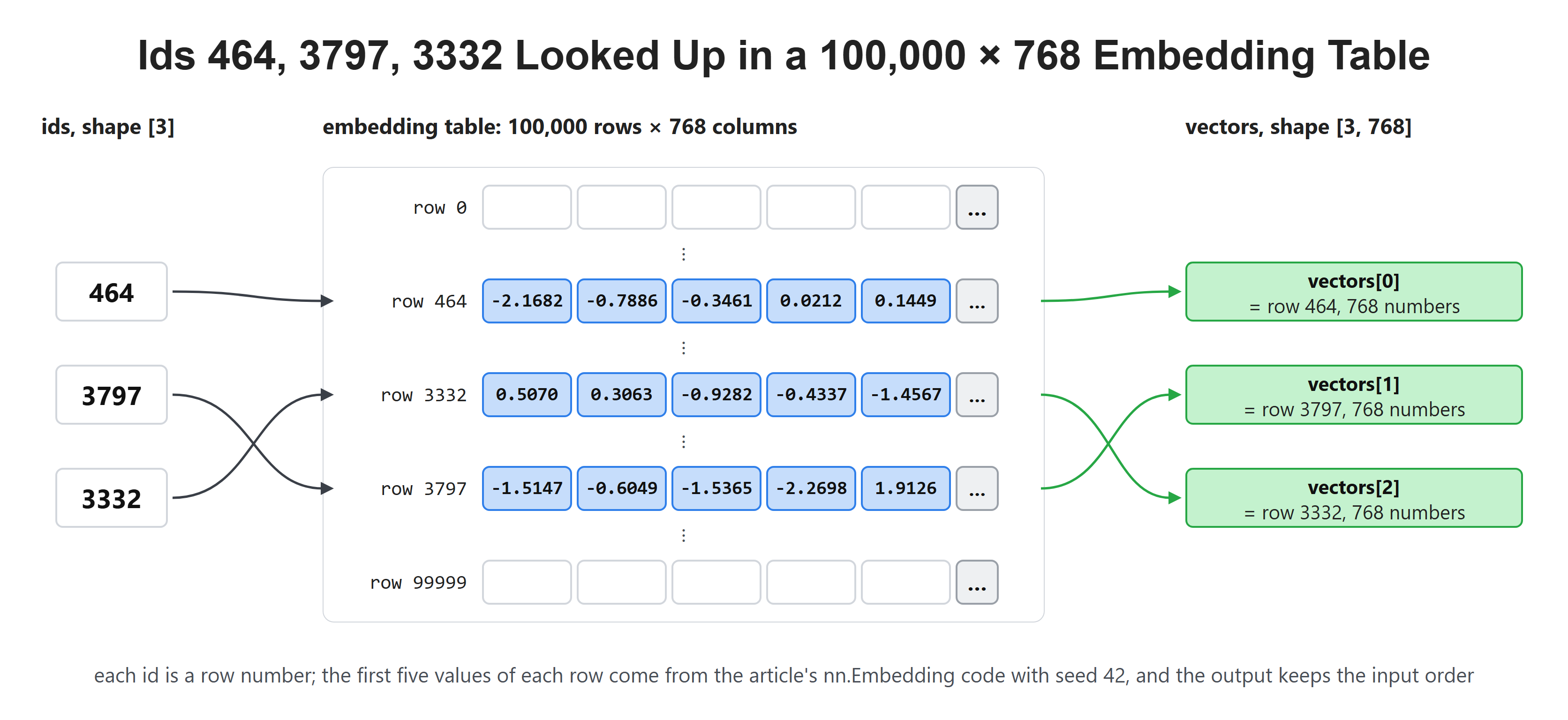
The real solution is a lookup table. The model keeps a big grid: one row per token in the vocabulary, and a fixed number of columns, often 768 or 4096.

To embed a token, the model does not compute anything clever. It goes to that token's row and reads it. The token ID is the row number, which is the only job the ID ever had.

In PyTorch that table is nn.Embedding. The two numbers it needs are the vocabulary size (how many rows) and the embedding dimension (how many columns).

import torch
import torch.nn as nn

torch.manual_seed(42)

# one row per token, 768 numbers per row
embedding = nn.Embedding(num_embeddings=100_000, embedding_dim=768)

ids = torch.tensor([464, 3797, 3332])

with torch.no_grad():
    vectors = embedding(ids)

print("ids shape     :", ids.shape)
print("vectors shape :", vectors.shape)
print("first 5 numbers of the cat row:", vectors[1][:5])

ids shape     : torch.Size([3])
vectors shape : torch.Size([3, 768])
first 5 numbers of the cat row: tensor([-1.5147, -0.6049, -1.5365, -2.2698,  1.9126])

Here, we can see the whole story in the shapes. Three IDs went in. A 3 × 768 block of numbers came out: one row of 768 values for each token. That is the trade the model makes: 768 numbers per token instead of one-hot's 100,000.

What the Numbers Mean

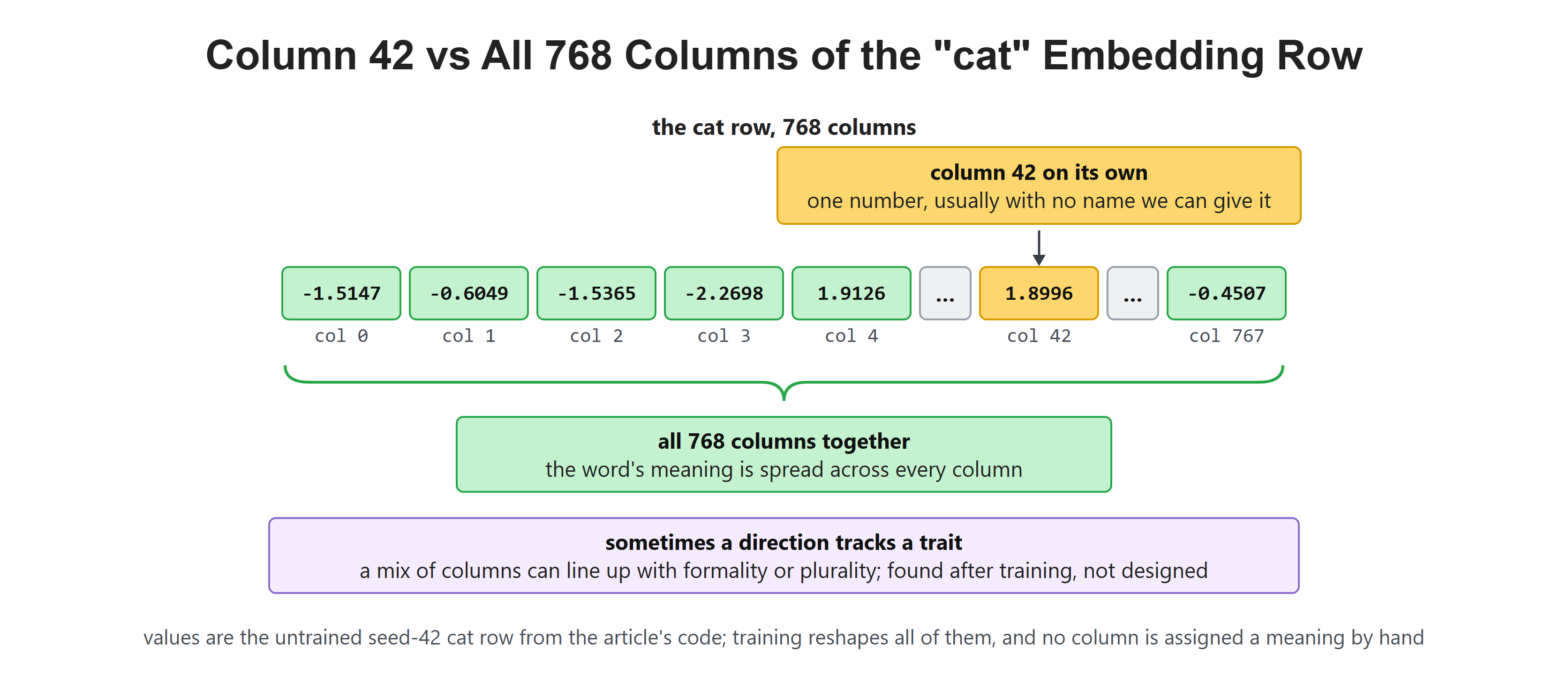
A natural question: what does the number in column 42 stand for? Usually nothing we can name.

The dimensions are not designed by hand. They are learned, and meaning is spread across all of them together rather than stored in any single one. Sometimes a direction turns out to track something we can recognise, like formality or plurality. But that is a discovery, not a design.

How Embeddings Learn Meaning

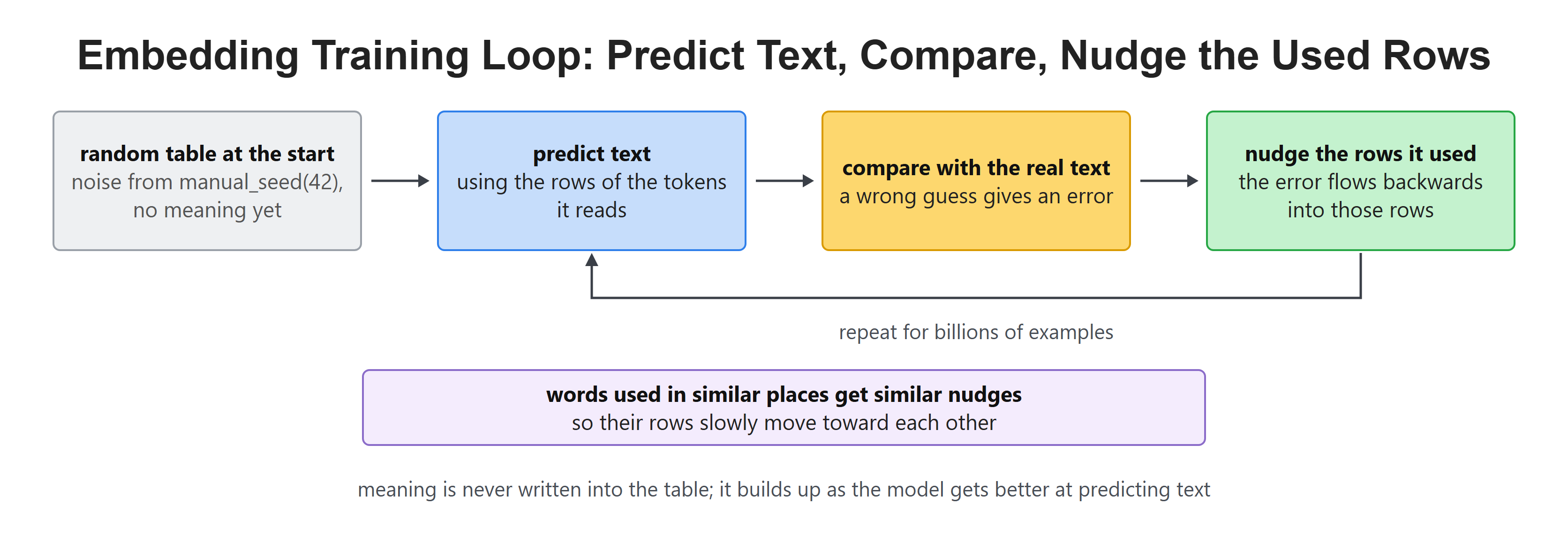
At the start of training, the whole table is random noise. Those numbers printed above are exactly that: noise from manual_seed(42). Nothing means anything yet.

Then training begins, and the model is repeatedly asked to predict text. Every time it gets something wrong, the error flows backwards and nudges the rows it used. Words that appear in similar places get nudged in similar directions, over and over, across the whole training set.

Meaning is not inserted. It accumulates, as a side effect of getting better at prediction.

Similar Words Drift Together

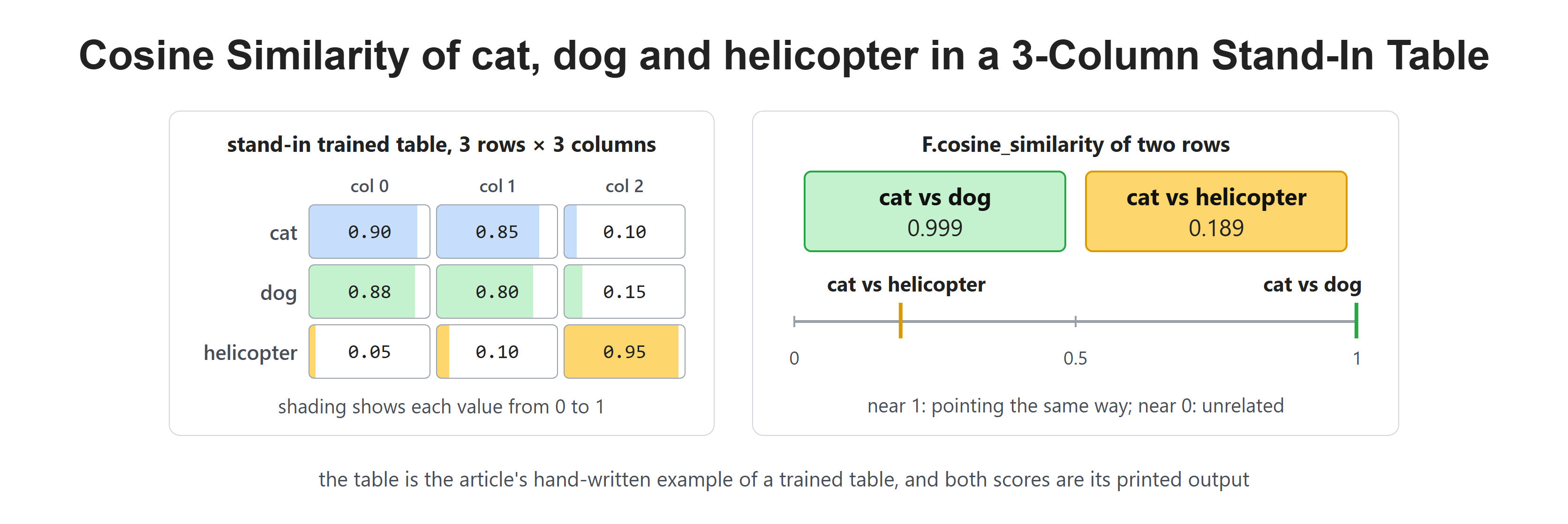
The result of all that nudging is the property that makes embeddings useful. Words used in similar contexts end up with similar vectors.

We cannot train a real model here. So we use a hand-written stand-in for a trained table: three words, three columns, with the two animals given similar rows. The usual way to compare two vectors is cosine similarity. It returns roughly 1 for "pointing the same way" and roughly 0 for "unrelated".

import torch
import torch.nn.functional as F

words = ["cat", "dog", "helicopter"]

# a tiny stand-in for a trained table: 3 rows, 3 columns
trained = torch.tensor([
    [0.90, 0.85, 0.10],   # cat
    [0.88, 0.80, 0.15],   # dog
    [0.05, 0.10, 0.95],   # helicopter
])

def similarity(a, b):
    return F.cosine_similarity(trained[a], trained[b], dim=0).item()

print("cat vs dog        :", round(similarity(0, 1), 3))
print("cat vs helicopter :", round(similarity(0, 2), 3))

cat vs dog        : 0.999
cat vs helicopter : 0.189

This is the number one-hot could never produce. "Cat" and "dog" appear near words like pet, feed, and vet, so their rows get pulled in similar directions. "Helicopter" is pulled elsewhere. Nobody told the model that cats and dogs are both animals; it fell out of the training text.

One Vector per Token, Not per Word

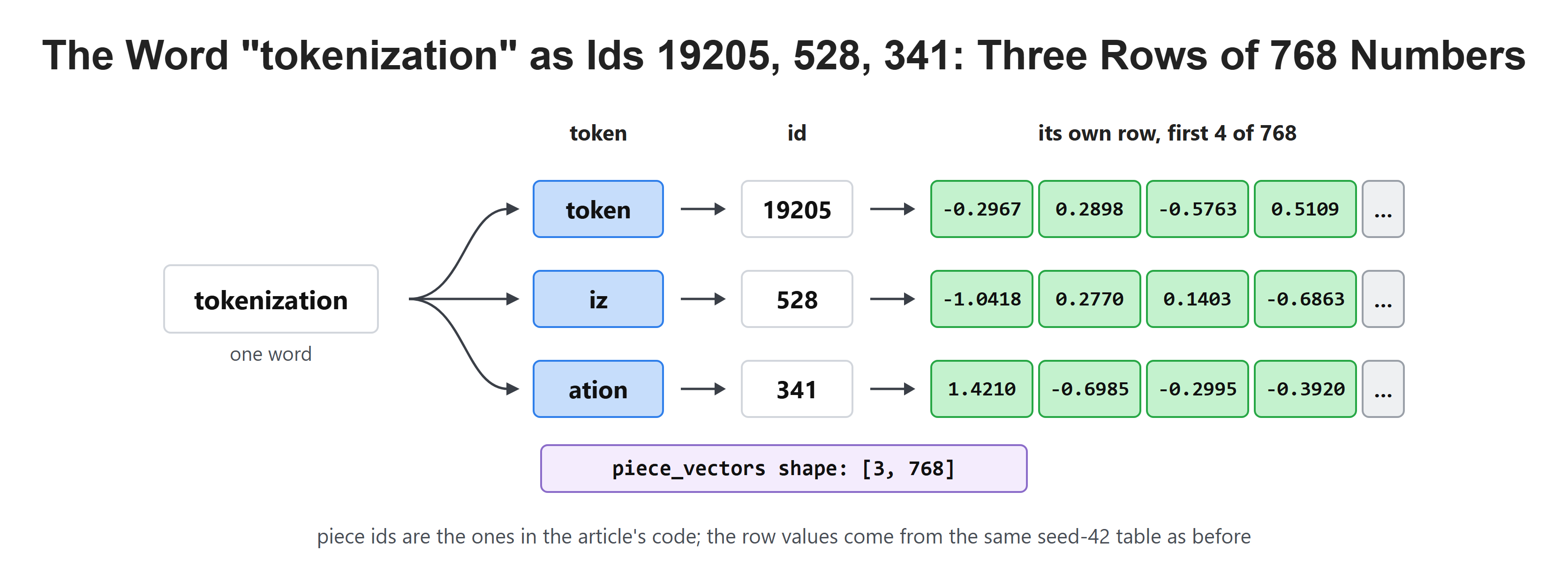
A detail that trips people up: embeddings are looked up per token, not per word. If a word splits into three tokens, it gets three separate vectors.

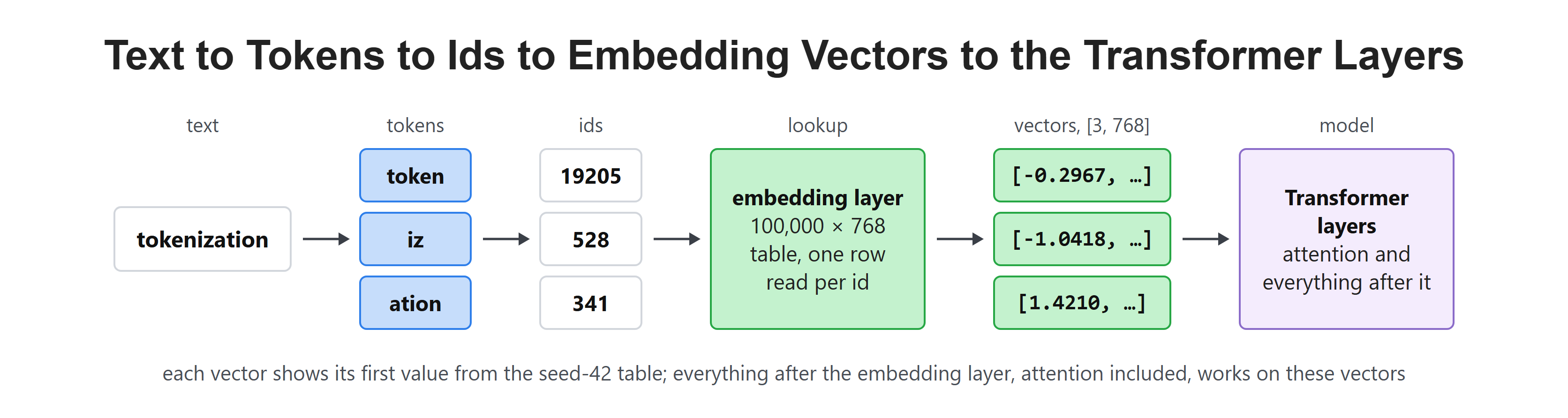
Let's reuse the same embedding layer from before and feed it three pieces of "tokenization". The IDs 19205, 528, and 341 for "token", "iz", and "ation" are example IDs, and the three-way split is only an example too. A real tokenizer may cut the word differently, for example into "token" and "ization".

# "tokenization" splits into three tokens, so it needs three lookups
piece_ids = torch.tensor([19205, 528, 341])   # token, iz, ation

with torch.no_grad():
    piece_vectors = embedding(piece_ids)

print("tokens :", piece_ids.shape[0])
print("shape  :", piece_vectors.shape)

tokens : 3
shape  : torch.Size([3, 768])

One word went in, three vectors came out. The later layers combine them. The embedding layer never sees whole words; it only sees the pieces the tokenizer produced.

Static at the Start, Contextual Later

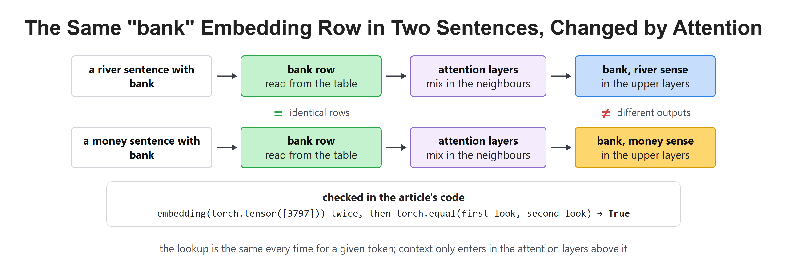
One more important point. The vector from the embedding table is the same every time for a given token. The row for "bank" does not change between a river sentence and a money sentence. The code below uses ID 3797 as a stand-in for any token, such as "bank":

with torch.no_grad():
    first_look  = embedding(torch.tensor([3797]))
    second_look = embedding(torch.tensor([3797]))

print("same vector both times?", torch.equal(first_look, second_look))

same vector both times? True

Context arrives afterwards, in the attention layers. They mix information between positions, so by the upper layers the representation of "bank" differs depending on its neighbours. The embedding is the starting point, not the final meaning.

Where Embeddings Sit in the Model

When we put it all together, the picture is simple. Text becomes tokens, tokens become IDs, IDs index the embedding table, and the resulting vectors are what actually flow into the Transformer.

Everything that follows, attention included, works on these vectors. The embedding layer is the doorway between language and mathematics.

Recap

This is how a token ID becomes meaning. The ID itself is only a row number, carrying no information about the word. One-hot encoding turns that ID into a vector. But as the code showed, it costs 390 KB per word and puts every pair of words at exactly the same distance.

The embedding table solves it: one row per token, a few hundred or few thousand numbers wide, and looking up a token is simply reading its row. Those numbers start as noise and are shaped by training. Words used in similar contexts drift toward similar vectors, and cosine similarity can measure how close they are. Each token gets its own vector, and that vector is the same every time until attention makes it contextual in the layers above.

In the next article, we treat these vectors as points in space and look at the geometry of meaning. We will see how similarity is measured, and what is really going on in the famous king minus man plus woman example.