Yesterday we ended with a table of numbers: one row per token, each row a few hundred values wide. Useful, but still abstract. Today those rows stop being lists and become locations.
Once a word is a point in space, questions about meaning turn into questions about geometry. Which points are close? Which way is it from man to woman? That shift is what makes search, clustering, and the famous analogy trick possible.
Note
The code below uses only NumPy: pip install numpy. Real embeddings have hundreds of dimensions, so to keep every number visible we use a hand-built toy space with four. The arithmetic is identical, just smaller.
A Vector Is a Point in Space
Two numbers describe a point on a page. Three describe a point in a room. Seven hundred and sixty-eight describe a point in a space nobody can picture, but the math works the same even when we cannot picture it.
Here is our toy space. Four dimensions, and for once we will say what each one means: how royal, how male, how female, how fruit.
import numpy as np

#                       royal  male  female  fruit
words = {
    "king":  np.array([0.95, 0.90, 0.05, 0.00]),
    "queen": np.array([0.95, 0.05, 0.90, 0.00]),
    "man":   np.array([0.10, 0.92, 0.05, 0.00]),
    "woman": np.array([0.10, 0.05, 0.92, 0.00]),
    "apple": np.array([0.02, 0.05, 0.05, 0.95]),
}

print("king  ->", words["king"])
print("queen ->", words["queen"])king -> [0.95 0.9 0.05 0. ]
queen -> [0.95 0.05 0.9 0. ]Read those two rows side by side. King and queen have the same first number, 0.95. On the next two numbers they swap places: king has 0.9 and 0.05, queen has 0.05 and 0.9. That pattern is the relationship between the words, written as coordinates.
In a real model nobody labels the columns. The dimensions are learned, and they mix concepts together. We label them here only so we can follow the arithmetic.
Direction, Not Length
The obvious way to compare two points is to measure the straight-line gap between them. For embeddings that turns out to be the wrong instinct.
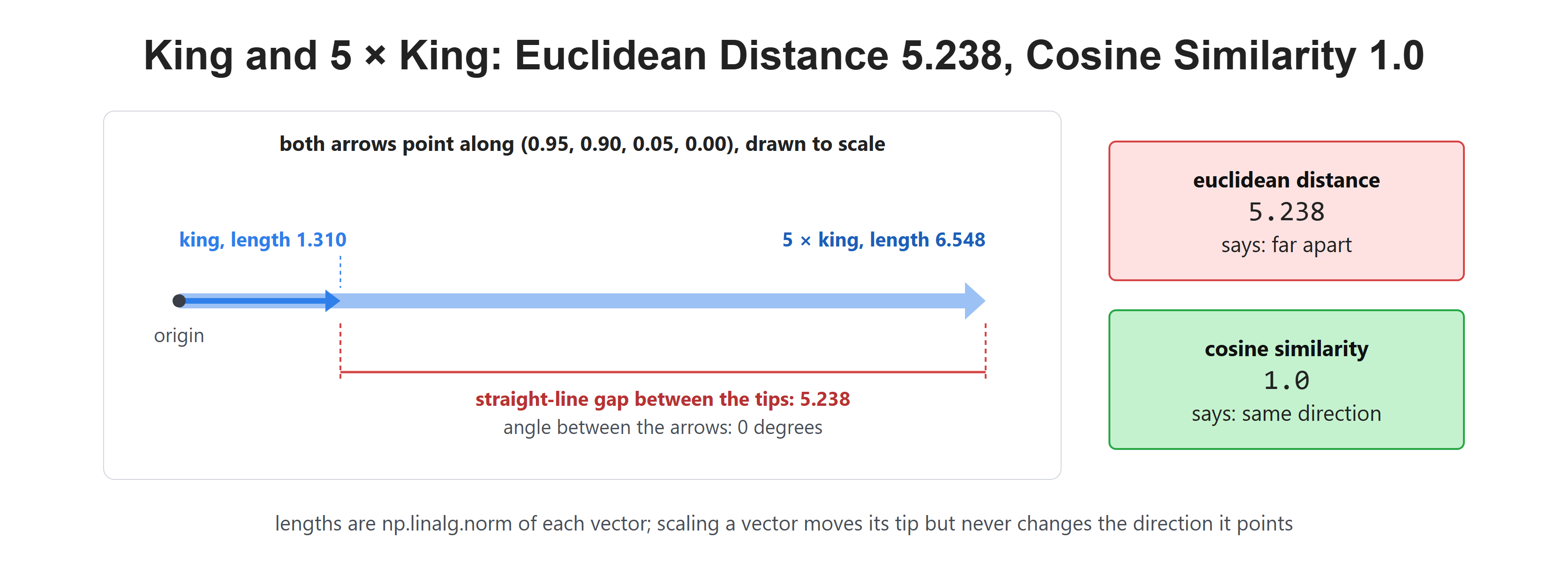
Watch what happens when we take king and simply make it five times longer, without changing which way it points.
king = words["king"]
long_king = king * 5

def cosine(a, b):
    return float(a @ b / (np.linalg.norm(a) * np.linalg.norm(b)))

print("euclidean distance :", round(float(np.linalg.norm(king - long_king)), 3))
print("cosine similarity :", round(cosine(king, long_king), 3))euclidean distance : 5.238
cosine similarity : 1.0Straight-line distance says these are far apart. Cosine says they are the same thing, and cosine is right: the vector points in exactly the same direction, it is just longer.
That matters because length can change while meaning stays the same, as the 5 × king test just showed. In real models, length is often linked to how often a word appeared in training. So a rare word and a common word can mean nearly the same thing while sitting at very different distances from the origin. Measuring the angle ignores length and keeps only the direction.
How Cosine Similarity Actually Works
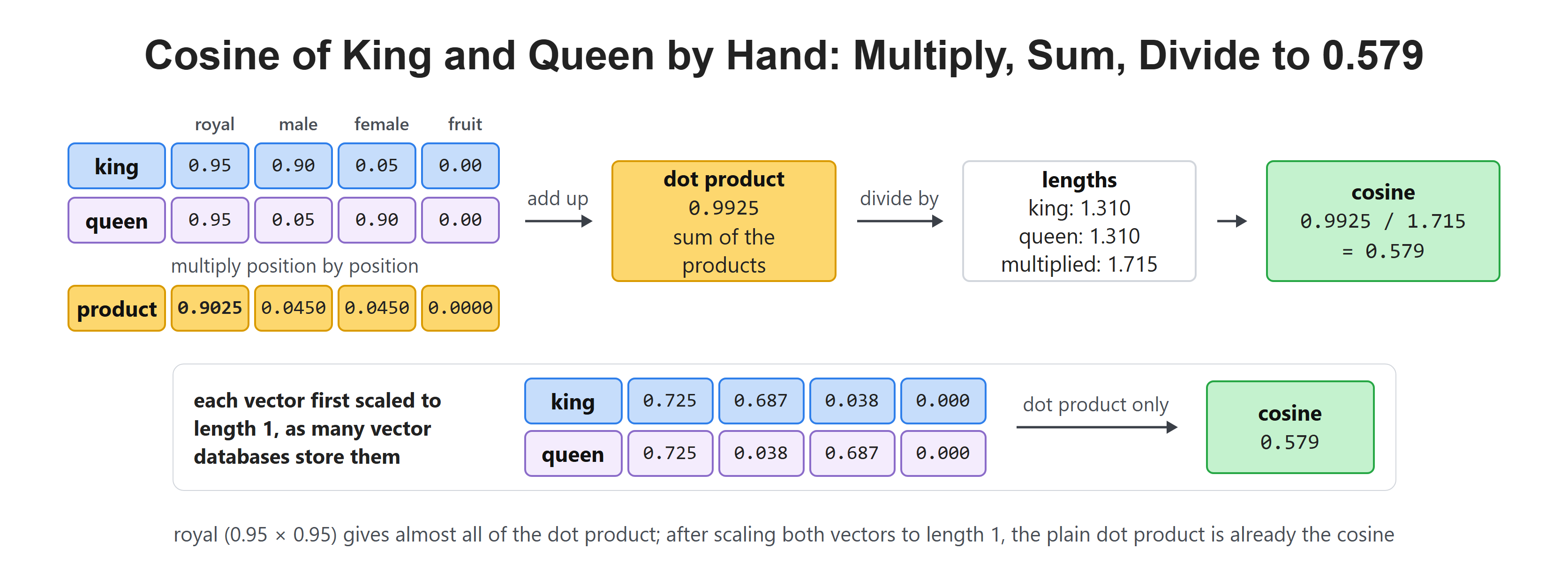
The formula has three pieces: multiply the two vectors position by position and add up the results, then divide by each vector's length.
Write it out once by hand so nothing is hidden behind a library call.
def cosine_from_scratch(a, b):
    dot = sum(x * y for x, y in zip(a, b))          # line up and multiply
    len_a = sum(x * x for x in a) ** 0.5            # length of a
    len_b = sum(y * y for y in b) ** 0.5            # length of b
    return dot / (len_a * len_b)

print("by hand :", round(cosine_from_scratch(words["king"], words["queen"]), 3))
print("numpy :", round(cosine(words["king"], words["queen"]), 3))by hand : 0.579
numpy : 0.579The dot product rewards dimensions where both words are large. King and queen are both high on royal, so that term contributes a lot. King is high on male where queen is near zero, so that term contributes almost nothing.
Dividing by the two lengths is what turns a raw score into a number between −1 and 1, so scores from different word pairs can be compared fairly.
Tip
Because dividing by length is the whole trick, many vector databases can normalise every vector to length 1 when storing it. After that, cosine similarity is just the dot product, so the division step is no longer needed on every comparison.
Reading a Similarity Table
One score on its own means little. Scores become readable when we rank them.
def rank_against(target, table):
    scores = [(name, round(cosine(target, vec), 3)) for name, vec in table.items()]
    return sorted(scores, key=lambda pair: pair[1], reverse=True)

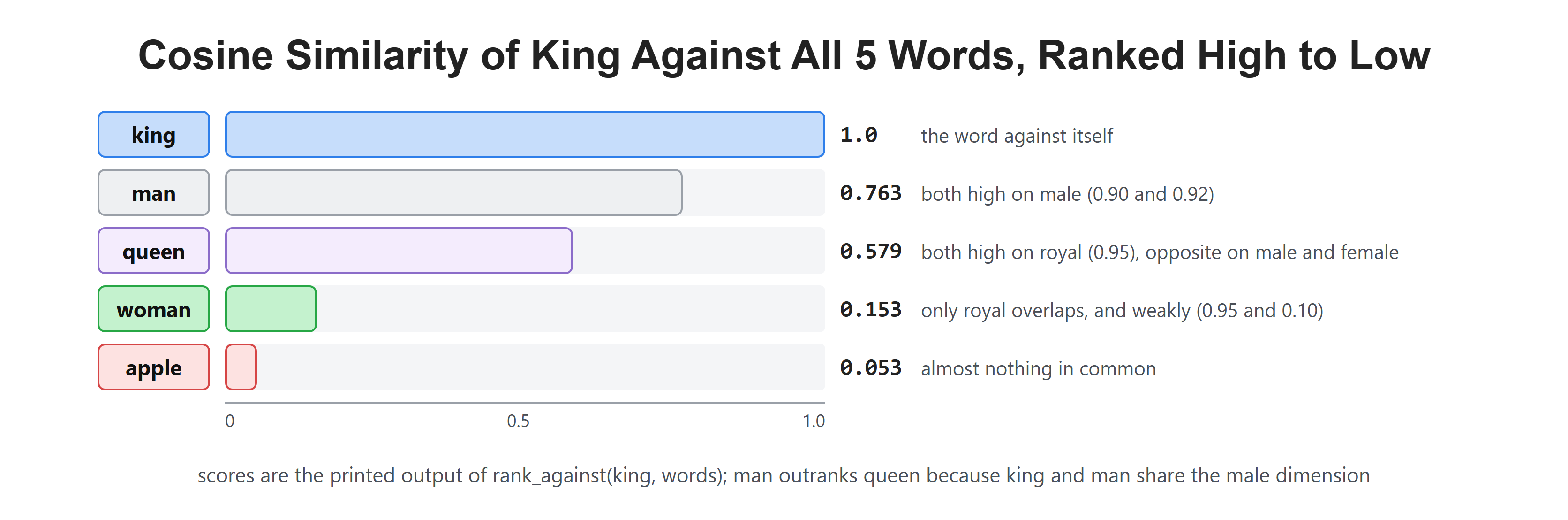
for name, score in rank_against(words["king"], words):
print(f"king vs {name:6s} {score}")king vs king 1.0
king vs man 0.763
king vs queen 0.579
king vs woman 0.153
king vs apple 0.053A word is always a perfect 1.0 against itself, which is a useful sanity check. Apple sits near zero, exactly as it should.
Now look at the middle of that list, because it is more interesting than it first appears. King is closer to man (0.763) than to queen (0.579). Nothing has gone wrong. King and man share a strong male dimension, while king and queen share royal but sit at opposite ends of two gender dimensions. "Similar" always means similar along the dimensions the model happens to have learned, which is not always the axis we had in mind.
Subtraction Gives You a Direction
Here is the idea the analogy trick rests on. Subtracting one vector from another does not give us a word. It gives us the step that takes us from the first to the second.
male_to_female = words["woman"] - words["man"]
king_to_queen  = words["queen"] - words["king"]

print("man    -> woman :", male_to_female)
print("king   -> queen :", king_to_queen)
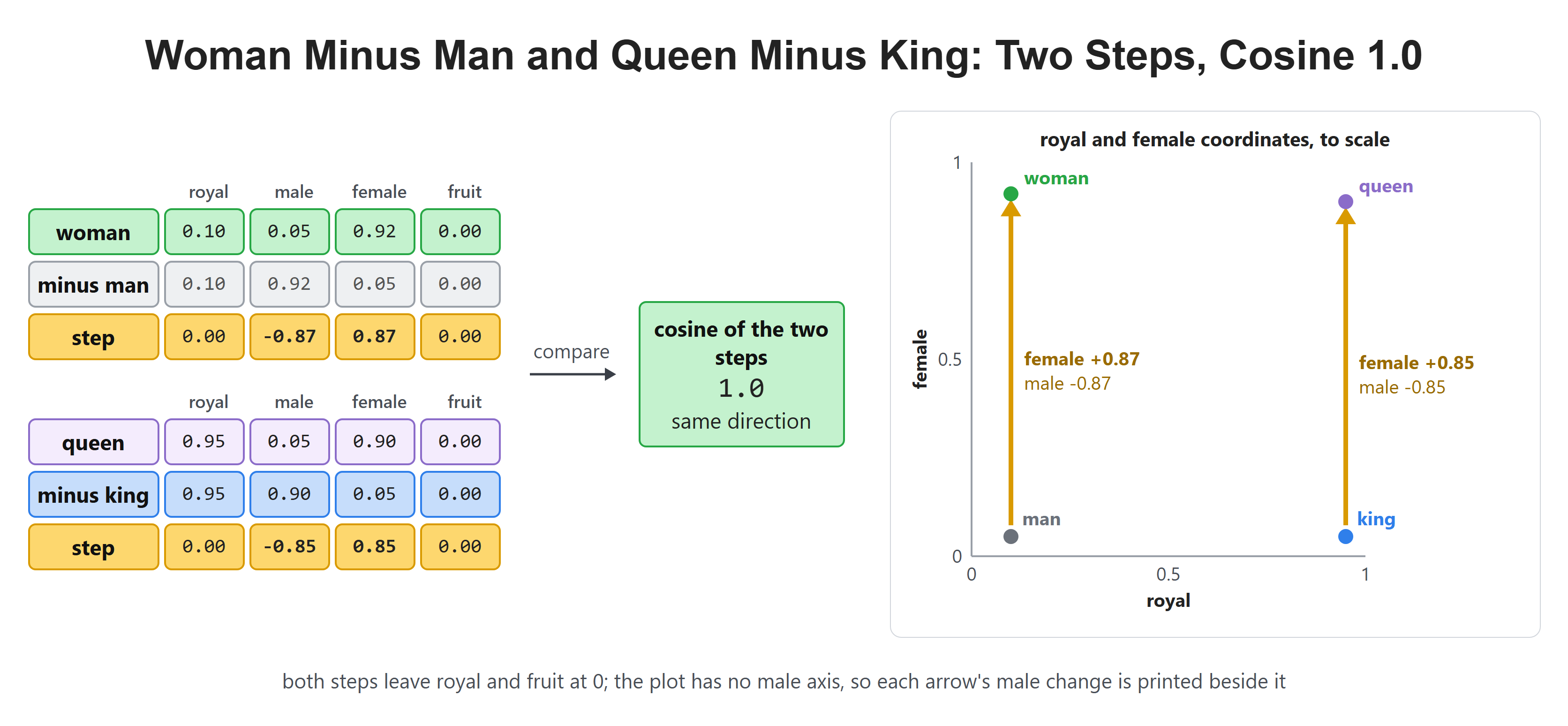
print("same direction? :", round(cosine(male_to_female, king_to_queen), 3))man -> woman : [ 0. -0.87 0.87 0. ]
king -> queen : [ 0. -0.85 0.85 0. ]
same direction? : 1.0Two different pairs of words, and almost the same step: drop the male dimension by 0.87 or 0.85, raise the female dimension by the same amount, leave everything else alone. Cosine confirms the two steps point the same way.
That shared step is what people mean when they say a "gender direction" exists in embedding space. In our toy space, we put it there by hand. In a real model, nobody programs it in. It can appear because the training text tends to use these word pairs in similar ways.
King Minus Man Plus Woman, Step by Step
Now the famous line. Read it as a journey rather than an equation: start at king, walk back along the male direction, then walk forward along the female direction, and see where we land.
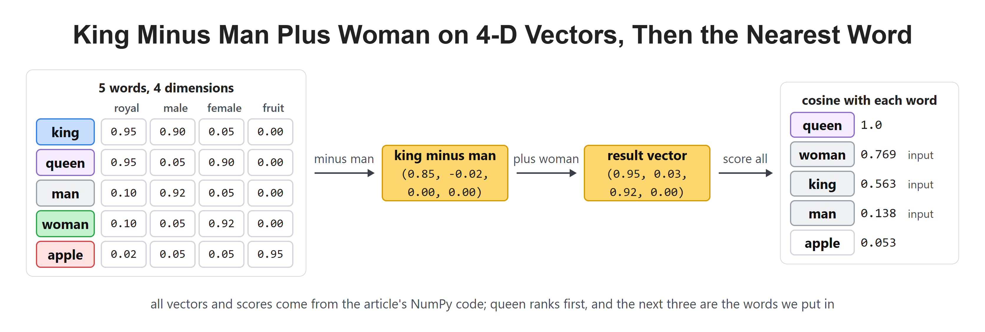
result = words["king"] - words["man"] + words["woman"]

print("start at king   :", words["king"])
print("minus man       :", words["king"] - words["man"])
print("plus woman      :", result)
print("queen looks like:", words["queen"])start at king : [0.95 0.9 0.05 0. ]
minus man : [ 0.85 -0.02 0. 0. ]
plus woman : [0.95 0.03 0.92 0. ]
queen looks like: [0.95 0.05 0.9 0. ]Follow the middle line, because that is where the work happens. Subtracting man knocks the male dimension from 0.90 down to −0.02 and wipes out the small female value, leaving a nearly pure royalty vector. It has stopped being a person and become a property. Adding woman then puts a person back, with the female dimension restored to 0.92.
The journey ends at [0.95, 0.03, 0.92, 0.00]. Queen sits at [0.95, 0.05, 0.90, 0.00]. Close, but not identical, and that gap matters for the next step.
The Answer Is a Nearest Neighbour, Not an Equation
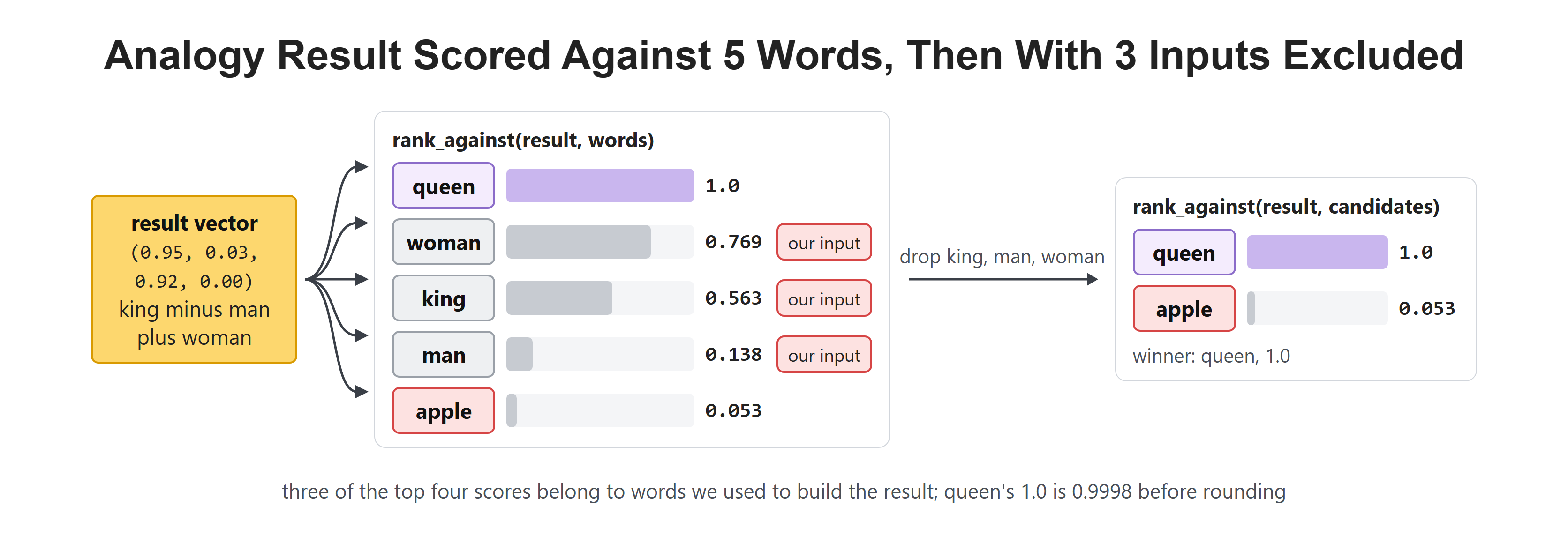
The result vector is not queen. It is a point near queen. So the last step of every analogy demo is a search: score the result against every word in the vocabulary and take the best match.
for name, score in rank_against(result, words):
print(f"result vs {name:6s} {score}")result vs queen 1.0
result vs woman 0.769
result vs king 0.563
result vs man 0.138
result vs apple 0.053Queen wins at 1.0, rounded from a fraction just under it. The demo works.
But look at second and third place. Woman scores 0.769 and king scores 0.563. Both are high, and both are words we put into the question ourselves. The answer sits near them because we built it out of them.
In our toy space, queen still beats them. In a real space, one of the input words can end up on top. That is why analogy searches commonly drop the three input words before naming a winner. Let's see the code as below:
inputs = {"king", "man", "woman"}
candidates = {w: v for w, v in words.items() if w not in inputs}

best = rank_against(result, candidates)[0]
print("excluding the inputs, the winner is:", best)excluding the inputs, the winner is: ('queen', 1.0)Here, we can see that the winner does not change. Queen already won the full search, so in our toy space the exclusion is only a safety step.
How Much This Really Proves
We need to be careful about what this shows.
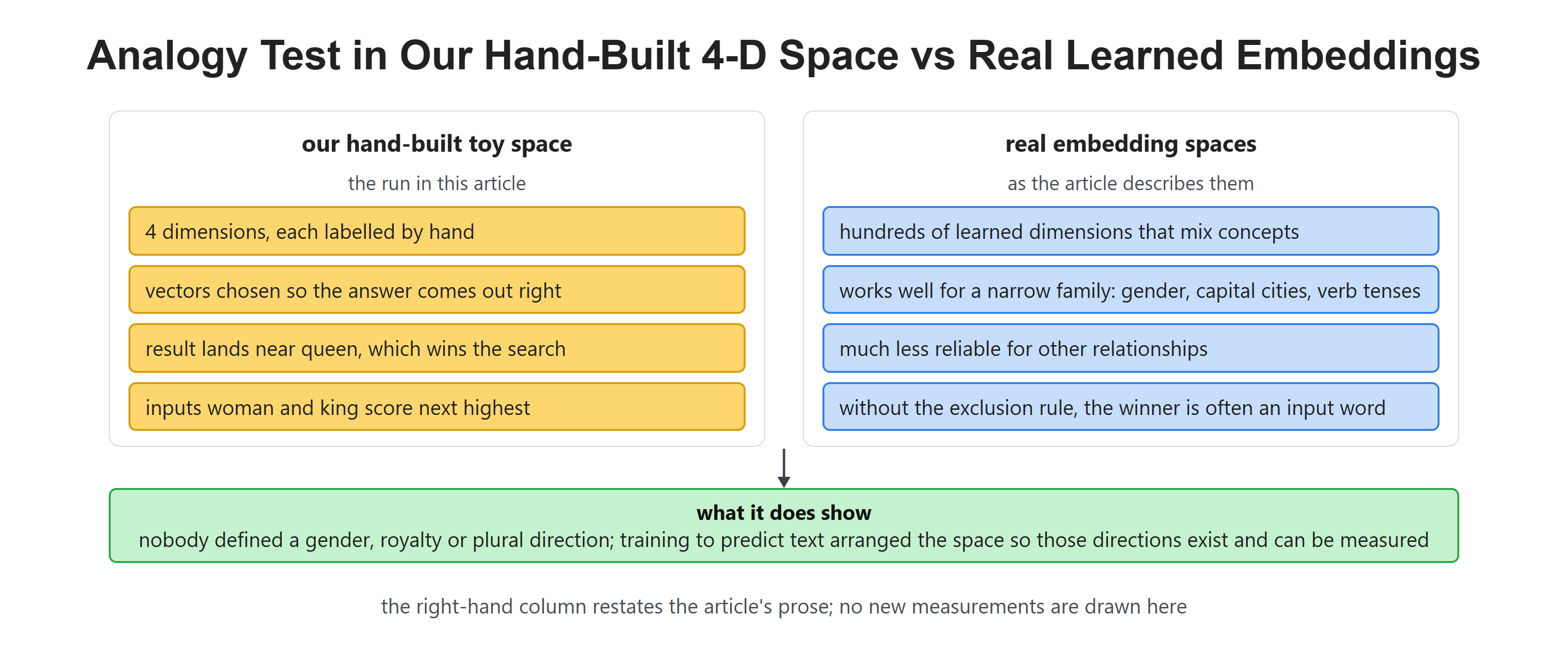
Our toy space was built by hand to make the answer come out right, so queen won even before we removed the input words. In real embedding spaces the picture is messier. The famous analogies are usually shown for a small set of relationships, such as gender, capital cities and verb tenses. They are often reported to work less well for others. And without the exclusion rule, the top match can turn out to be one of the input words itself.
So the honest summary is smaller than the headline. In a real model, nobody defines a gender, royalty, or plural direction. Training the model to predict text arranges the space, and directions like these can then be found and measured.
Where This Geometry Gets Used
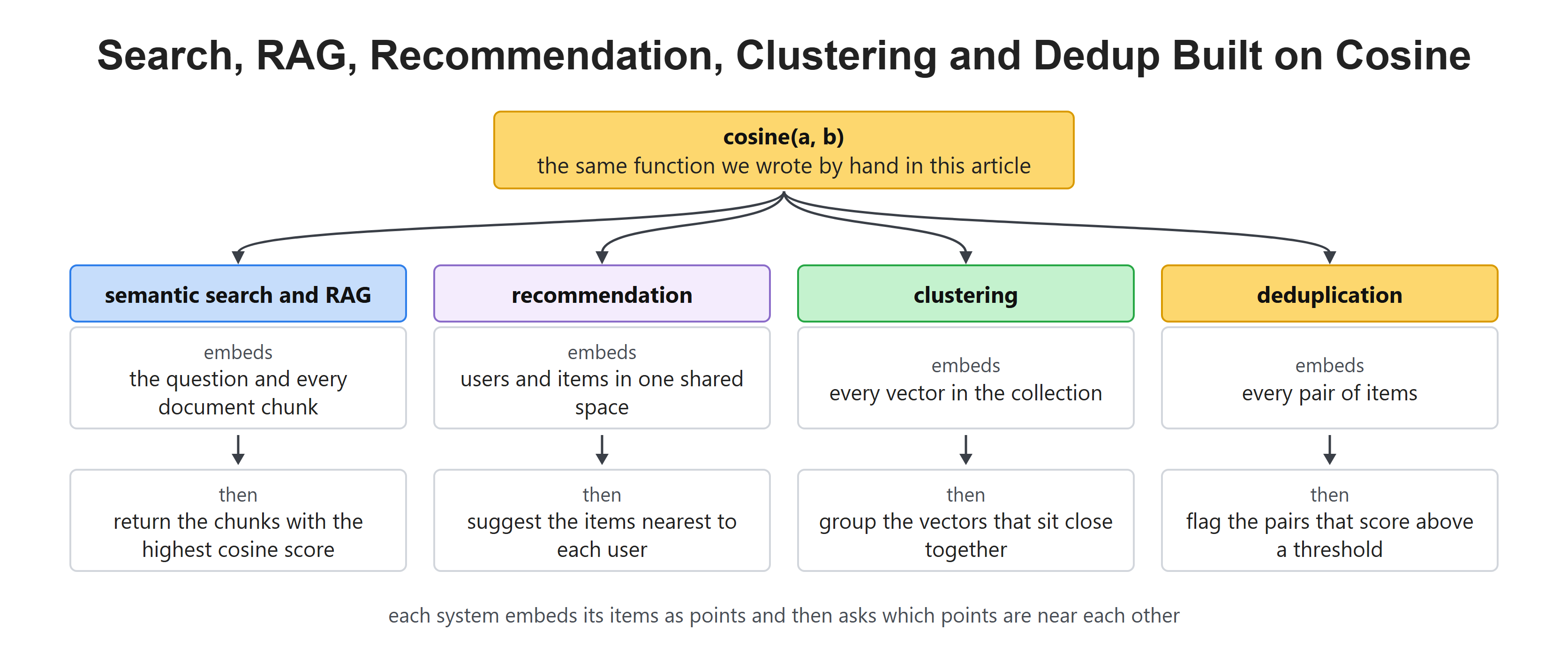
This geometry is not only a demo. Many everyday systems run on it.
Semantic search and RAG embed the question and every document, then return the chunks with the highest cosine score. Recommendation systems place users and items in one space and look for near neighbours. Clustering groups vectors that sit together. Deduplication flags pairs above a threshold. Every one of those is the same operation we just wrote by hand.
This is why we spent today on geometry. Once meaning is a location, "find me something similar" becomes "find me something nearby". And finding nearby points is a job computers do well.
Recap
This is how the geometry of meaning works. An embedding is a point in space, and the geometry of that space carries the meaning. Straight-line distance is the wrong ruler because length can change while meaning stays the same. Cosine similarity measures the angle instead and returns a comparable score between −1 and 1.
Subtracting two vectors gives a direction rather than a word. In our toy space, the same direction turned up between man and woman and between king and queen. That shared step is what makes analogies possible at all. King minus man plus woman lands near queen, but "near" is the key word. The final step is a nearest-neighbour search. In our toy space queen wins it with or without the input words. In real spaces, the input words are usually dropped from the search first.
That geometry is what semantic search, RAG retrieval, recommendation, and clustering all run on. In the next article we leave single vectors behind and ask why a sentence needs more than a bag of points, which is the problem attention was invented to solve.