
Knowing what people think about a film, or any product, at scale is one of the most common real-world machine learning tasks. Sentiment analysis is the process of automatically detecting whether a piece of text expresses a positive or negative opinion. Rather than reading thousands of reviews by hand, we train a model to do it for us.
In this blog, we build a complete sentiment classifier from scratch. We load 50,000 IMDB movie reviews, clean the text, convert it into numerical vectors using TF-IDF (Term Frequency-Inverse Document Frequency), and train a Linear SVM (Support Vector Machine) to label each review as pos or neg. Along the way we learn how to evaluate the classifier and save it for production use.
Prerequisites: Python 3.x, Pandas, NumPy, scikit-learn, spaCy, BeautifulSoup4, TextBlob.
Setting Up the Environment
Install the core libraries before running any code:
!pip install pandas
!pip install numpy
!pip install scikit-learn
Import Pandas (the table-based data analysis library) and NumPy (the numerical array library):
import pandas as pd
import numpy as np
Loading the Dataset
The IMDB dataset contains 50,000 reviews split into a Reviews column (raw text) and a Sentiment column (pos or neg). Clone it from GitHub using git clone:
!git clone https://github.com/laxmimerit/IMDB-Movie-Reviews-Large-Dataset-50k.gitCloning into 'IMDB-Movie-Reviews-Large-Dataset-50k'...Read the training split into a Pandas DataFrame:
df = pd.read_excel('IMDB-Movie-Reviews-Large-Dataset-50k/train.xlsx')TF-IDF Vectorization
Machine learning models cannot read text directly: every word must become a number. TF-IDF is the standard technique for this. It scores each word by how often it appears in a document (term frequency) divided by how common it is across all documents (inverse document frequency). Rare but meaningful words like "masterpiece" score higher than common filler words like "the".
The diagram below illustrates the TF-IDF formula with its component parts labeled:
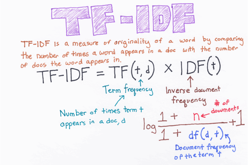
The formula is:
Where:
- : the term (word) being scored
- : the document (review) containing the term
- : the number of times term appears in document
- : the total number of documents in the corpus
- : the number of documents that contain term
In practice, a word like "beautiful" scores much higher than "is" because "is" appears in almost every document (making its IDF close to zero), while "beautiful" is selective.
Import the vectorizer, model, and evaluation utilities we need:
from sklearn.feature_extraction.text import TfidfVectorizer
from sklearn.model_selection import train_test_split
from sklearn.svm import LinearSVC
from sklearn.metrics import classification_report
Inspect the first five rows to confirm the column layout:
# show first 5 rows
df.head()| Reviews | Sentiment | |
|---|---|---|
| 0 | When I first tuned in on this morning news, I ... | neg |
| 1 | Mere thoughts of "Going Overboard" (aka "Babes... | neg |
| 2 | Why does this movie fall WELL below standards?... | neg |
| 3 | Wow and I thought that any Steven Segal movie ... | neg |
| 4 | The story is seen before, but that does'n matt... | neg |
Text Preprocessing
Raw user reviews contain noise: HTML tags, email addresses, URLs, and exaggerated repeated characters (e.g., "looooove") that add no signal to the model. We need to strip all of that before vectorizing.
Install the preprocess_kgptalkie package, which bundles all the cleaning helpers used here:
!pip install git+https://github.com/laxmimerit/preprocess_kgptalkie.gitThe package depends on spaCy, BeautifulSoup4, and TextBlob. Install them first:
!pip install spacy==2.2.3
!python -m spacy download en_core_web_sm
!pip install beautifulsoup4==4.9.1
!pip install textblob==0.15.3
Import the preprocessing module and Python's built-in regular expression library:
import preprocess_kgptalkie as ps
import re
The docstring below describes each cleaning step that get_clean applies:
"""
Step 1: Lowering the letter then after replacing backward slash from nothing and underscore from space.
Step 2: Remove emails from the Reviews column.
Step 3: Removing html tags from the Reviews column.
Step 4: Removing special character.
Step 5: If you have multiple repeated character then it converted into single character and make meaningful.
E.g. x = 'lllooooovvveeee youuuu'
x = re.sub("(.)\1{2,}", "\1", x)
print(x)
-------
love you
"""
Define the get_clean function and apply it to every row in the Reviews column:
def get_clean(x):
    x = str(x).lower().replace('\\', '').replace('_', ' ')
    x = ps.cont_exp(x)
    x = ps.remove_emails(x)
    x = ps.remove_urls(x)
    x = ps.remove_html_tags(x)
    x = ps.remove_accented_chars(x)
    x = ps.remove_special_chars(x)
    x = re.sub("(.)\\1{2,}", "\\1", x)
    return x

df['Reviews'] = df['Reviews'].apply(lambda x: get_clean(x))
df.head()| Reviews | Sentiment | |
|---|---|---|
| 0 | when i first tuned in on this morning news i t... | neg |
| 1 | mere thoughts of going overboard aka babes aho... | neg |
| 2 | why does this movie fall well below standards ... | neg |
| 3 | wow and i thought that any steven segal movie ... | neg |
| 4 | the story is seen before but that doesn matter... | neg |
Upper-case letters, HTML artefacts, and punctuation are gone. The text is now uniform and ready to vectorize.
Fit the TfidfVectorizer on the cleaned reviews, keeping only the 5,000 most informative words (max_features=5000):
tfidf = TfidfVectorizer(max_features=5000)
X = df['Reviews']
y = df['Sentiment']

X = tfidf.fit_transform(X)
X'
with 2843804 stored elements in Compressed Sparse Row format>The result is a sparse matrix. Most of its 2.8 million stored values are zero, because each review uses only a small fraction of the 5,000-word vocabulary. Sparse storage keeps memory usage manageable.
Split the dataset into 80 % training and 20 % test sets:
X_train, X_test, y_train, y_test = train_test_split(X, y, test_size = 0.2, random_state = 0)Support Vector Machine Classifier
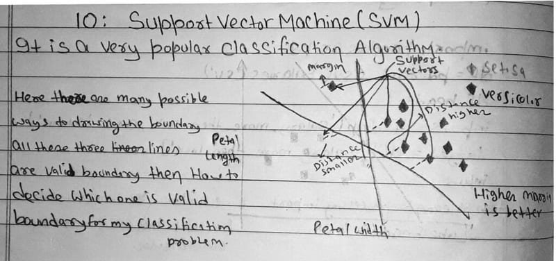
A Support Vector Machine (SVM) is a supervised learning algorithm that finds the hyperplane, a decision boundary in high-dimensional space, that separates two classes with the widest possible margin. The data points closest to the boundary on each side are called support vectors. Maximising the gap between them is what makes SVMs robust against noise.
The diagram below shows how the SVM chooses between multiple valid boundaries by picking the one with the highest margin:
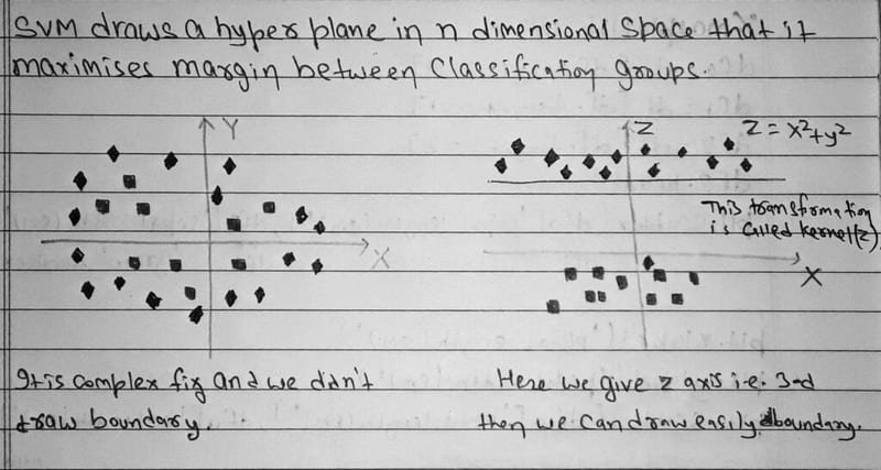
When data is not linearly separable in two dimensions, the kernel trick maps it into a higher-dimensional space where a flat hyperplane can separate the classes. The diagram below illustrates this: data that cannot be split by a line in 2D becomes separable once a third axis is added:
LinearSVC is a fast linear-kernel SVM optimised for large text datasets. It finds the hyperplane that best separates positive from negative reviews in the 5,000-dimensional TF-IDF space. Fit it on the training set and generate predictions:
clf = LinearSVC()
clf.fit(X_train, y_train)
y_pred = clf.predict(X_test)Evaluating the Classifier
A classification report breaks down performance by class. Precision measures how many of the predicted positives were actually positive. Recall measures how many actual positives were correctly identified. F1-score is the harmonic mean of the two.
print(classification_report(y_test, y_pred)) precision recall f1-score support
neg 0.87 0.87 0.87 2480
pos 0.87 0.88 0.88 2520
accuracy 0.87 5000
macro avg 0.87 0.87 0.87 5000
weighted avg 0.87 0.87 0.87 5000The classifier reaches 87 % accuracy, with balanced precision and recall on both classes. It is equally reliable at detecting negative and positive reviews; neither class is systematically ignored.
Predicting on New Text
To verify the model on a custom sentence, pass it through the same cleaning pipeline and then transform it with the fitted vectorizer before calling predict:
x = 'this movie is really good. thanks a lot for making it'

x = get_clean(x)
vec = tfidf.transform([x])
Check the shape of the resulting feature vector. It should have exactly 5,000 columns, one per vocabulary word:
vec.shape(1, 5000)Predict the sentiment label:
clf.predict(vec)array(['pos'], dtype=object)The model correctly labels the enthusiastic review as positive.
clf.predict(vec)array(['pos'], dtype=object)Saving the Model with Pickle
Pickle serializes Python objects, converting them to a byte stream, so we can write them to disk and reload them later without retraining. Save both the classifier and the vectorizer (we need both at inference time):
import pickle
pickle.dump(clf, open('model', 'wb'))
pickle.dump(tfidf, open('tfidf', 'wb'))
Both files are now on disk. To use them in a deployment script, call pickle.load() on each file, then call tfidf.transform() and clf.predict() exactly as we did above.
Conclusion
In this blog, we built a complete end-to-end sentiment classifier for IMDB movie reviews. We cleaned raw text with preprocess_kgptalkie, converted it to a 5,000-feature TF-IDF matrix, and trained a LinearSVC that achieved 87 % accuracy with balanced precision and recall across both classes. Finally, we saved the trained model and vectorizer to disk using pickle.
Key takeaways:
- TF-IDF down-weights common words and up-weights rare but meaningful words, giving the SVM better signal to learn from.
LinearSVCis a fast, high-quality baseline for text classification. It handles the high-dimensional sparse output ofTfidfVectorizerefficiently.- The preprocessing step matters as much as the model: removing HTML tags, URLs, and repeated characters directly improves the quality of the learned vocabulary.
- We must save both the vectorizer and the classifier. New text must pass through the same
tfidf.transform()call before prediction. - Balanced precision and recall (both ~0.87) confirms the model is not biased toward one class.
Next steps:
- Try Multi-label Text Classification on Stack Overflow to extend these techniques to problems with more than two output classes.
- Explore Real-time Sentiment Analysis of a Phone Call using NLTK and TextBlob to see how sentiment scoring works on streaming audio transcripts.
- Read SVM with Python for a deeper look at how Support Vector Machines work with different kernels and on non-text datasets.