On Day 13, we gave every word a query, key, and value. A query asks, "Which information do I need?" A key says, "What kind of information do I offer?" A value carries the information that can be passed on. Now we need the exact rule that connects those three pieces.
That rule is scaled dot-product attention. It scores keys against a query, turns the scores into weights, then uses those weights to blend value vectors.
This first diagram shows the order of those operations before we inspect each one.
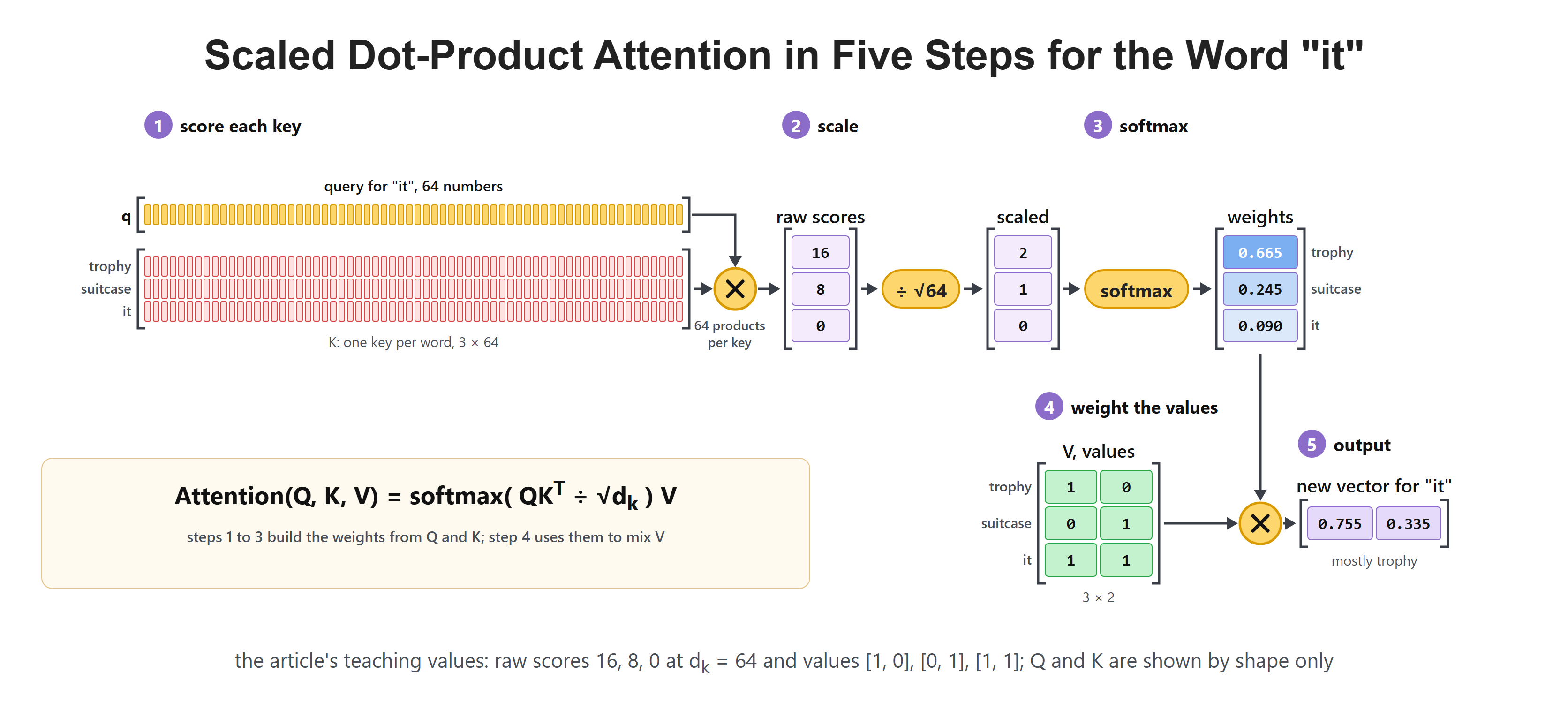
Attention scores query-key matches, scales the scores, normalizes them with softmax, and uses the result to mix values.
:::note We use three words and 64-value vectors in this lesson. Real models are often wider, but 64 is large enough to make the scaling problem visible. :::
The Formula, Read One Part at a Time
The complete rule is short:
Do not try to read it all at once. Read it from the inside out.
- is the matrix of query vectors.
- is the matrix of key vectors.
- is the matrix of value vectors.
- means that the key matrix is turned sideways.
- is the number of values in one key vector.
First, compares every query with every key. Next, division by controls the size of those comparison scores. Softmax changes each score row into weights. Finally, multiplying by takes a weighted blend of the values.
For the rest of this article, we follow the word it in a sentence with trophy, suitcase, and it. Suppose it's query gives these raw scores:
| Key | Raw score from it's query |
|---|---|
| trophy | 16 |
| suitcase | 8 |
| it | 0 |
The trophy is the best match, and suitcase may still add useful context. The question is how to turn those three scores into a sensible amount of attention.
Keep Track of the Shapes
For three query positions and three key positions, and each have shape . Transposing gives . The two inner dimensions match, so has shape . Its rows belong to queries and its columns belong to keys.
Our values will have only two features each, so has shape . A weight matrix multiplied by returns a output. Query and key widths must match, but value width need not equal key width. The output width follows the values.
The scores in this lesson are invented to make the arithmetic visible. We are not claiming that a trained model actually gives the word "trophy" a score of 16. The same distinction applies to the diagrams: they explain a calculation, not a measured attention map.
Why Wider Vectors Produce Bigger Scores
A dot product multiplies matching vector positions and then adds all those products. With four positions, it adds four small terms. With 64 positions, it adds 64 terms. Positive and negative terms may partly cancel, but the usual size of the total still grows as we add more positions.
Under a useful starting assumption, query and key entries are independent, have mean zero, and have variance one. Variance measures the average squared spread around the mean. Each product then has variance one, and adding such products gives variance . The standard deviation, the square root of variance, grows as . Learned vectors need not keep these exact statistics. With , that number is . This growth does not mean that the model suddenly found a better match. It happens partly because the vector is wider.
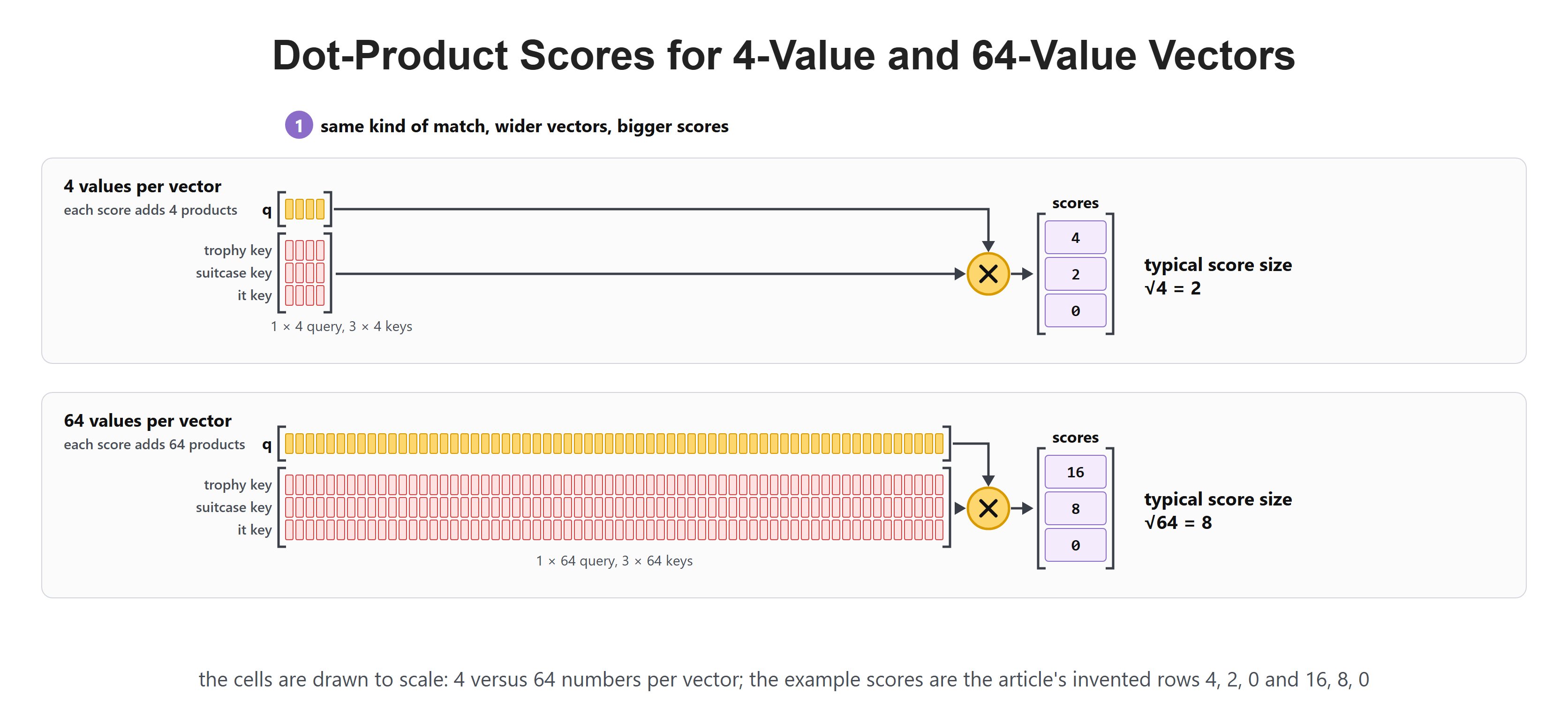
Adding more products makes raw dot-product scores larger even when the kind of match has not changed.
Here is a small comparison. The order of the scores remains useful. The trouble is the scale of the scores before softmax sees them.
| Key size | Example raw scores | Typical score size |
|---|---|---|
| 4 | 4, 2, 0 | 2 |
| 64 | 16, 8, 0 | 8 |
If raw scores become too large, softmax reacts very strongly to even a modest difference. That can make attention pick almost one key just because vectors are wide.
Softmax Turns Scores into Weights
Raw scores are not weights. A raw score can be negative, and three raw scores do not have to add to one. We need a set of positive numbers that says how much each value should contribute.
Softmax does that job. For a score in a row, it uses:
The exponential makes every number positive. Dividing by the total makes all weights in that row add to one. A larger score still receives a larger weight.
The next diagram shows why our raw row [16, 8, 0] is too sharp when it reaches softmax unchanged.
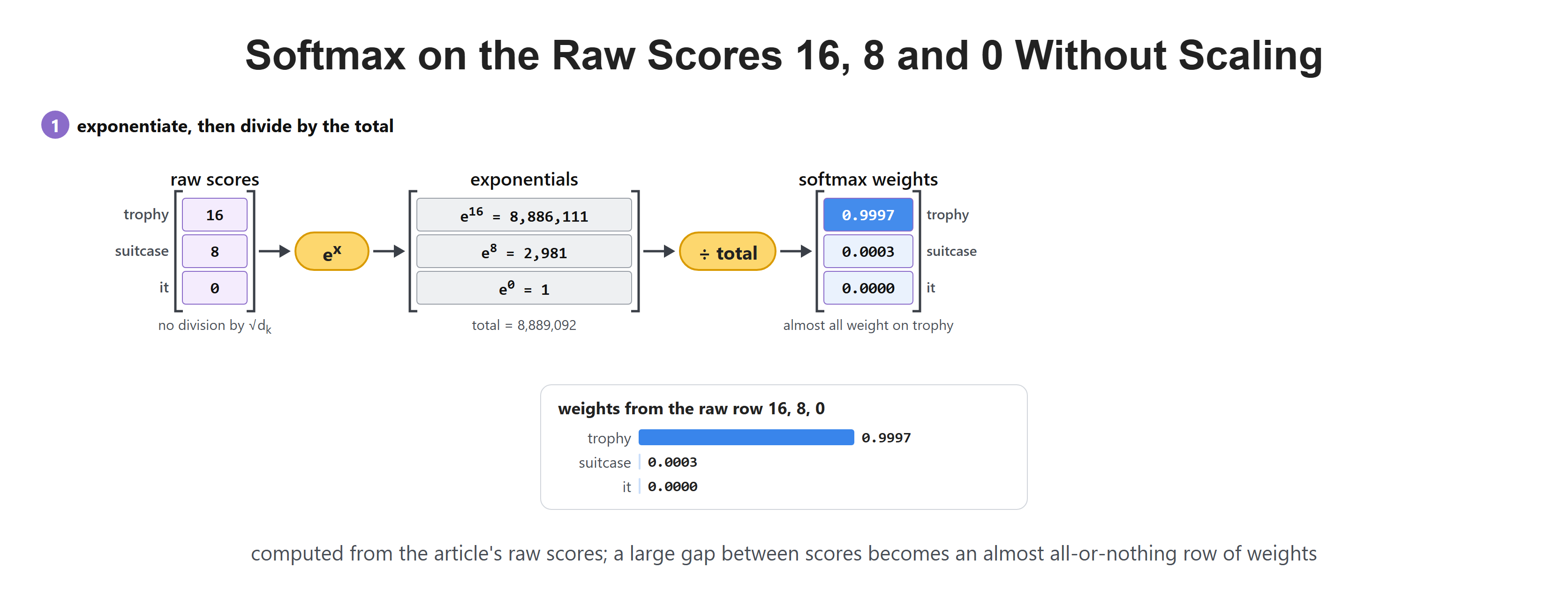
A large raw-score gap becomes an almost all-or-nothing attention distribution after softmax.
If we use softmax directly, the result is close to this:
| Key | Raw score | Weight after raw softmax |
|---|---|---|
| trophy | 16 | 0.9997 |
| suitcase | 8 | 0.0003 |
| it | 0 | 0.0000 |
Trophy clearly wins, but suitcase has almost no way to pass information forward. A near-one weight can be correct when the learned match is truly overwhelming. This invented score row shows what a large score gap does; the numbers alone do not prove that vector width caused the gap.
To see what softmax is doing, take a small score row, exponentiate every entry, and divide each result by their sum. The calculation gives a probability-like row of weights, not a new set of meanings.
Why We Divide by the Square Root of d
The scaling step repairs the size problem before softmax. Our key size is 64, and . So we divide every score in the row by 8:
We have not changed the winner. Trophy is still ahead of suitcase, and suitcase is still ahead of it. We have only returned the scores to a range where softmax can express a useful preference.
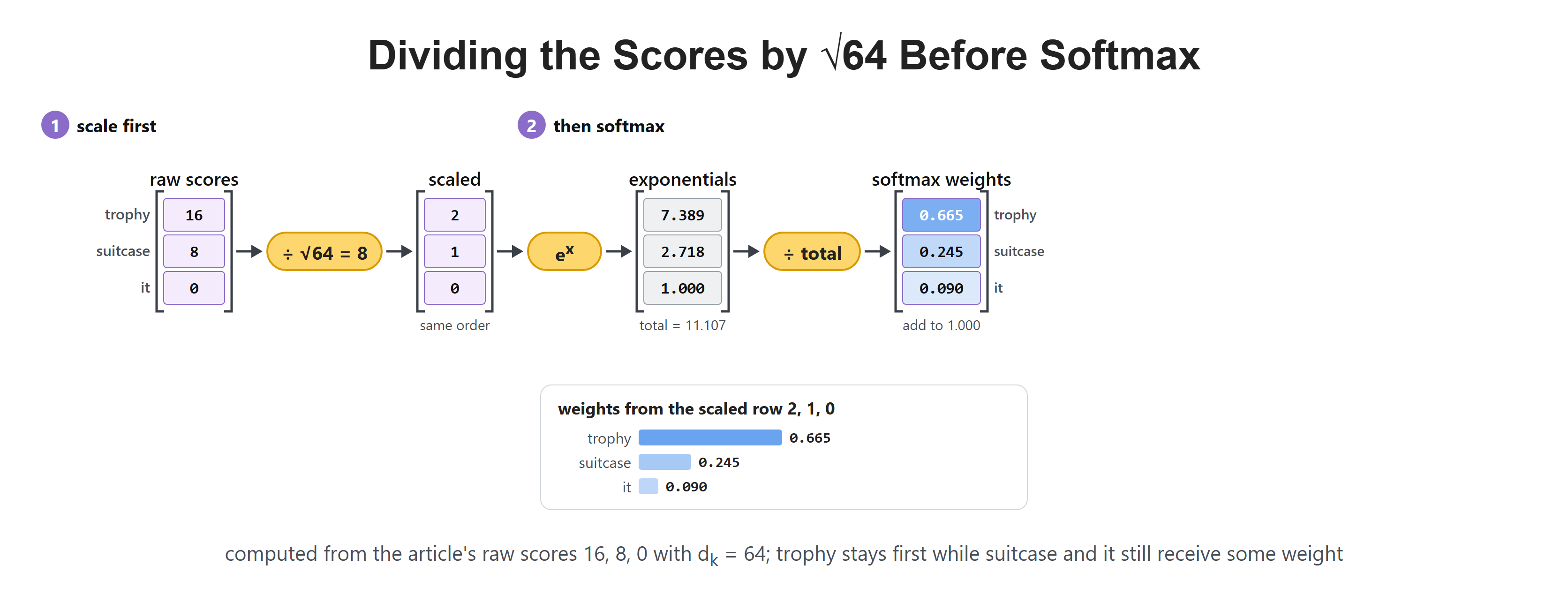
Dividing by controls the usual score growth before softmax makes weights.
Now softmax gives a more informative distribution:
| Key | Scaled score | Weight after softmax |
|---|---|---|
| trophy | 2 | 0.665 |
| suitcase | 1 | 0.245 |
| it | 0 | 0.090 |
Trophy still supplies most of the information. Suitcase can now supply some context, and the word itself retains a small amount. This is a preference, not an accidental forced winner.
Why divide by the square root rather than by 64? Dividing by 64 would turn [16, 8, 0] into [0.25, 0.125, 0]. Softmax would then produce weights that are nearly even. That throws away a real preference.
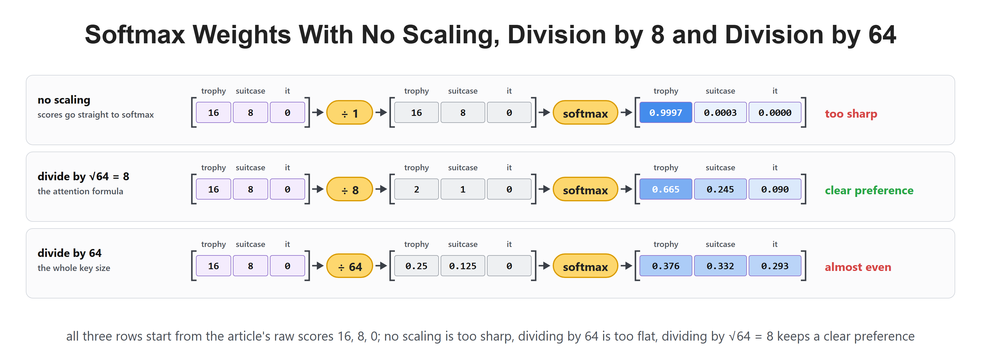
No scaling is too sharp here, while dividing by the whole key size makes the distribution too flat.
The square root matches the usual growth of a dot product. It reduces the unwanted growth without erasing the model's learned score differences.
A score difference matters through a ratio. For scores 2 and 1, the ratio of their unnormalized weights is , about 2.72. For scores 16 and 8, that ratio is , about 2,981. This is why keeping the ranking unchanged does not keep the distribution unchanged.
Very sharp attention is not always wrong. The training concern is that an almost-one weight leaves little room for the distribution to respond to small score changes. For softmax, a weight's derivative with respect to its own score is . That quantity is small near both zero and one. Scaling helps avoid this saturation at the start of training; it does not guarantee good learning by itself.
An attention weight is a mixing coefficient, not a probability that a word is true, relevant in a human sense, or the cause of the answer. We should read 0.665 as "use this fraction of the value in this head's mixture," not "the model is 66.5% certain about trophy."
Values Carry the Information
The weights do not mix the keys. Keys were only used to decide where to look. The final weights mix values, because values hold the information to send to the next layer.
Let trophy's value be [1, 0], suitcase's value be [0, 1], and it's value be [1, 1]. Using the scaled weights from above gives:
The output is mostly trophy information, with smaller contributions from suitcase and it. That blended vector is the new context-aware representation for it.
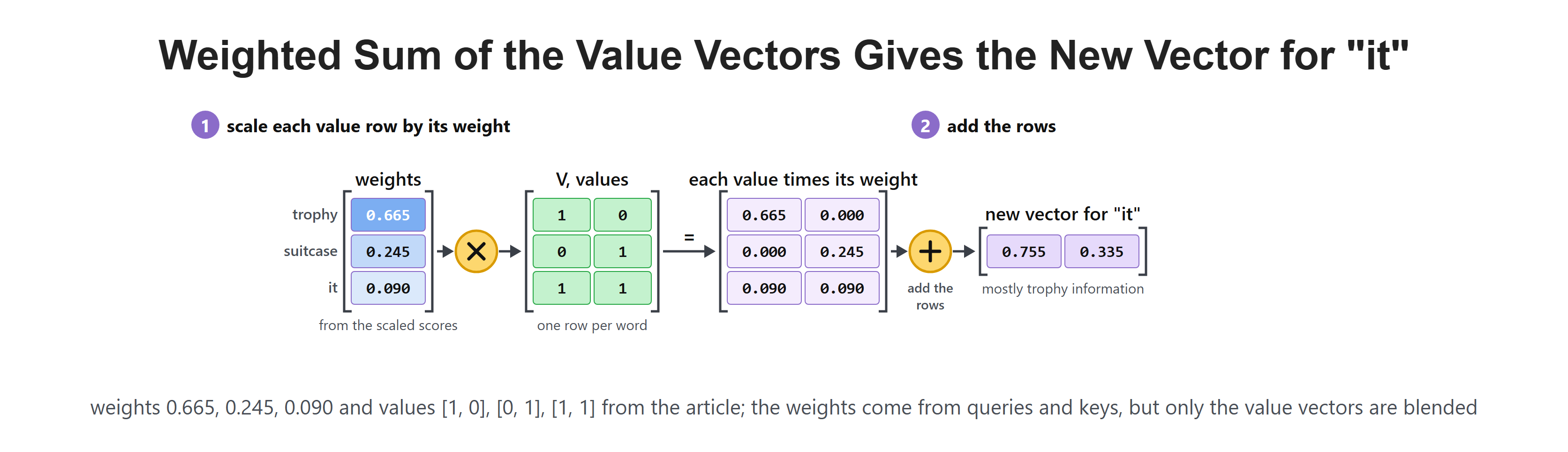
Queries and keys decide the weights; the weighted values form the attention output.
Every Word Gets Its Own Score Row
We followed only it's query, but every word has a query. For three words, creates a three-by-three score grid. Each row belongs to one query, and softmax works across one row at a time.
| Query word | trophy key | suitcase key | it key |
|---|---|---|---|
| trophy | 8 | 4 | 0 |
| suitcase | 4 | 8 | 0 |
| it | 16 | 8 | 0 |
The third row is our example. The first two rows are the questions asked by trophy and suitcase. Matrix multiplication calculates all these comparisons efficiently in one operation.
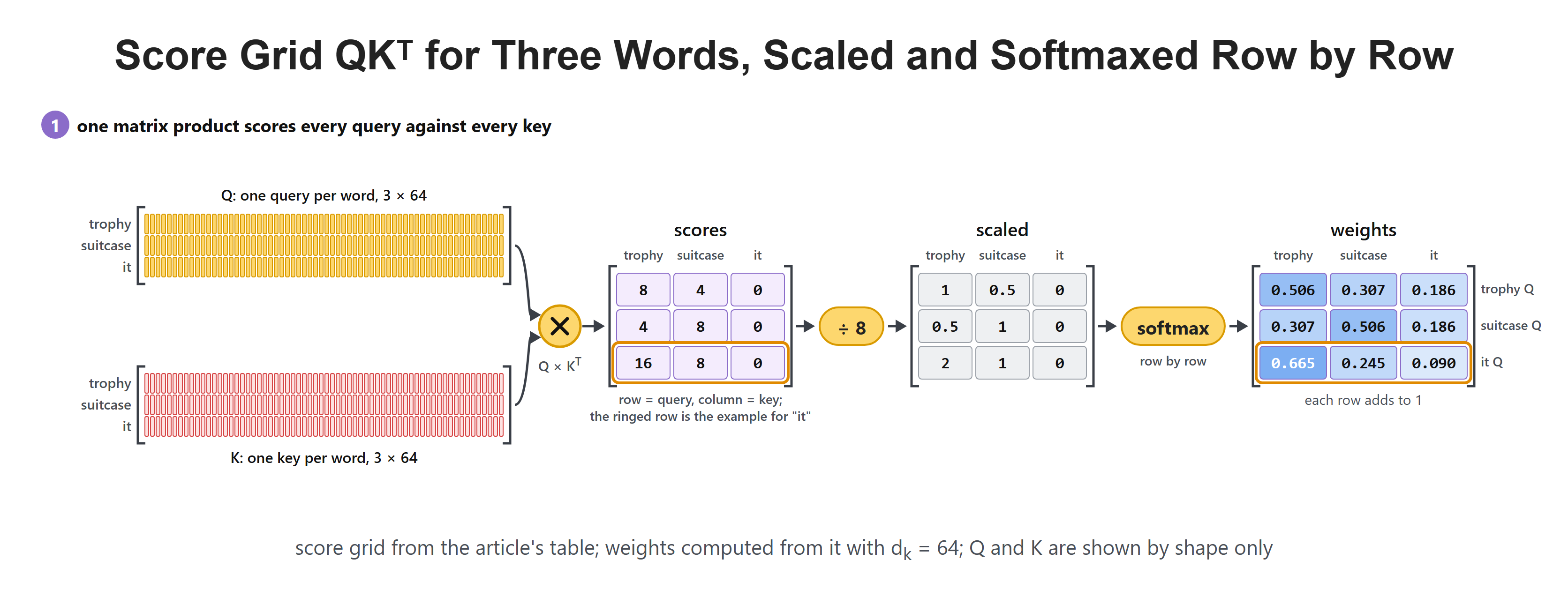
Each row asks one word's question about all keys in the sequence.
A Small Step That Keeps Softmax Safe
Real implementations often subtract the largest score in each row before applying softmax. For [16, 8, 0], subtracting 16 produces [0, -8, -16].
This does not change the final weights. Every exponential is divided by the same shared total, so moving every score by the same amount cancels out. It does prevent very large exponentials from causing number problems in code.
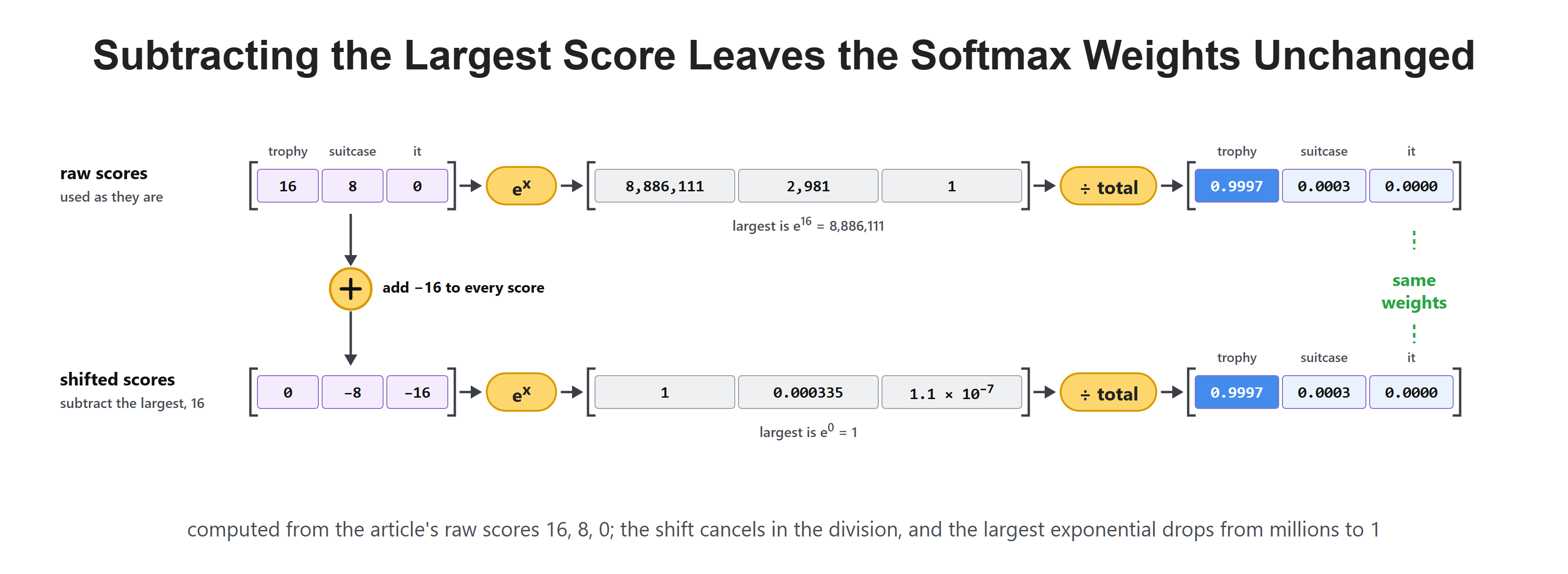
Subtracting the row maximum keeps the computation safe while leaving the softmax weights unchanged.
Check the Same Row in NumPy
NumPy lets us calculate the row without building a Transformer. We first import it, then define the already-computed dot products and key width.
import numpy as npThe width is 64 because that is the number of products in each query-key score. It is not the number of tokens or the width of our teaching values.
raw_scores = np.array([16.0, 8.0, 0.0])
key_width = 64
scaled_scores = raw_scores / np.sqrt(key_width)
Subtract the maximum after scaling. Subtracting a shared constant leaves softmax unchanged, while dividing changes its sharpness. These two operations solve different problems.
exponentials = np.exp(scaled_scores - scaled_scores.max())
weights = exponentials / exponentials.sum()
values = np.array([[1.0, 0.0], [0.0, 1.0], [1.0, 1.0]])
context = weights @ values
The weights are approximately [0.665241, 0.244728, 0.090031]. The context is approximately [0.755272, 0.334759]. The first coordinate receives contributions from trophy and it; the second receives contributions from suitcase and it.
Check two properties before changing the example: the weights sum to one, and there is one weight per value row. Replacing a value changes the mixed output but does not change the weights. Replacing a key can change the weights because keys participate in the scores.
The Full Attention Step
For one query position, the complete attention process is now easy to state:
- Compare its query with all keys to get raw scores.
- Divide by to control score size.
- Apply softmax across that score row.
- Use the resulting weights to add value vectors.
Recap
Scaled dot-product attention starts with query-key scores. Softmax turns those scores into weights, but wide vectors make raw dot products grow and can make softmax sharp for the wrong reason. Dividing by keeps the scale useful.
The weights choose how much each value contributes. On Day 15, we will run several attention calculations in parallel so different heads can learn different relationships in the same sentence.