In Day 19, we met the full Transformer block. It had attention, an MLP, two shortcut additions, and a norm. The norm got only a few short paragraphs. But here's the real mystery: if we remove it, a deep model can fail to train. So what is this small layer doing?
A normalization layer rescales the numbers inside one token vector so they stay at a steady size. In simple words, it stops every layer's input from getting too big or too small. In this lesson, we will learn why LLMs need it, how LayerNorm and RMSNorm work, where the norm sits in the block, and what QK-Norm adds inside attention.
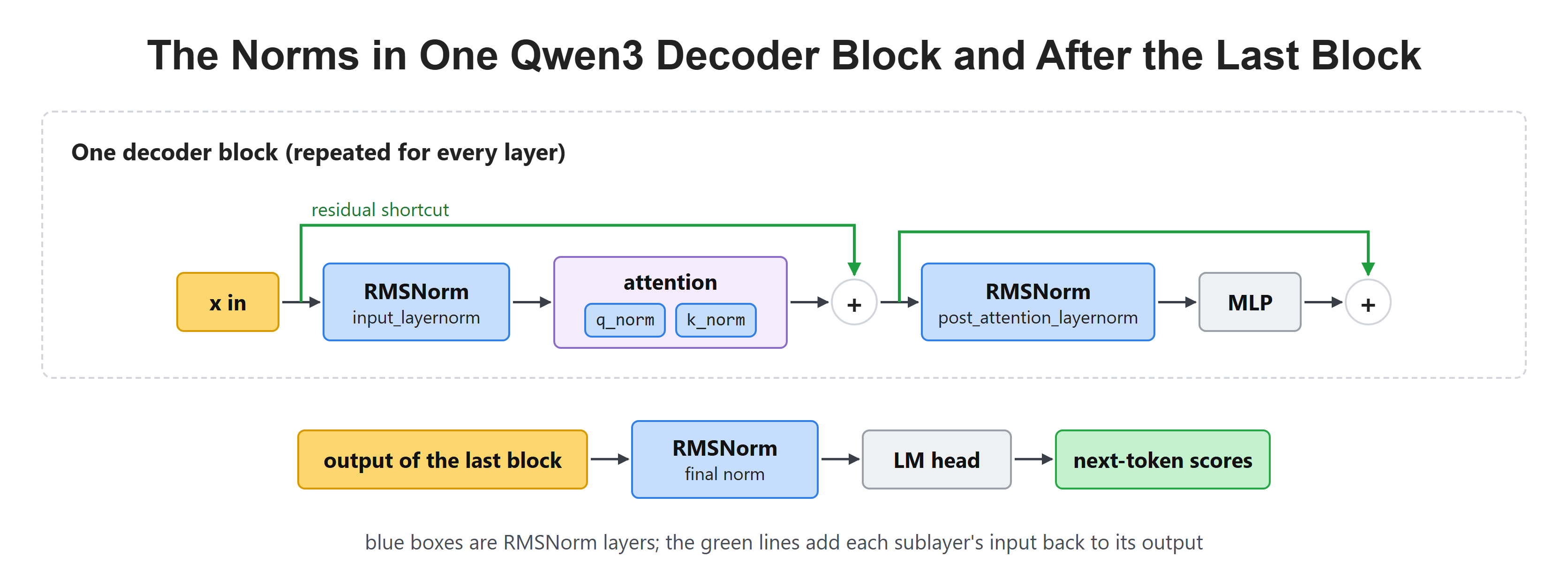
Every blue box is an RMSNorm. By the end of this lesson, we will know why each one sits where it does.
Why Does a Deep Transformer Need a Norm?
Let's start with the problem. In Day 19, we saw that each block adds its result back to its input. This running vector is called the residual stream. Every block reads it, works on it, and adds something to it.
Now, an LLM stacks many blocks. Qwen2.5-0.5B has 24 of them. If every block makes the numbers a little bigger, the growth piles up. Block 24 then sees numbers far larger than block 1 saw. Its weights were never tuned for inputs that big, so training becomes shaky.
Let's see this with a tiny toy. We build 24 random layers, each 512 numbers wide, with a shortcut around each one. We run the same input through two copies. One copy feeds each layer the raw stream. The other copy rescales the stream first. Let's see the code as below:
import torch

torch.manual_seed(0)
d, depth = 512, 24
layers = [torch.randn(d, d) / d ** 0.5 for _ in range(depth)]

def rms(v):
    return v.pow(2).mean().sqrt().item()

def norm(v):
    return v / v.pow(2).mean().sqrt()

x_plain = torch.randn(d)
x_norm = x_plain.clone()

for i, W in enumerate(layers, start=1):
    seen_plain = x_plain
    seen_norm = norm(x_norm)
    x_plain = x_plain + W @ seen_plain
    x_norm = x_norm + W @ seen_norm
    if i in (1, 6, 12, 24):
print(f"layer {i:2d}: no norm sees {rms(seen_plain):8.1f} with norm sees {rms(seen_norm):.1f}")layer 1: no norm sees 1.0 with norm sees 1.0
layer 6: no norm sees 5.6 with norm sees 1.0
layer 12: no norm sees 45.9 with norm sees 1.0
layer 24: no norm sees 2738.7 with norm sees 1.0Here, we can see the problem clearly. Without a norm, layer 24 sees inputs of size 2,738.7. With a norm, every layer sees size 1.0.
A few choices in this code are worth a word:
- We divide the random weights by
d ** 0.5so one layer keeps the size of its input about the same. Even so, the shortcut adds the input back, so the size still grows a little at every layer. - The
rmshelper measures the size of a vector. RMS stands for root mean square: square every number, take the mean, then take the square root. - The
normhelper divides a vector by its own RMS. This is a bare RMSNorm, which we will meet properly in a moment.
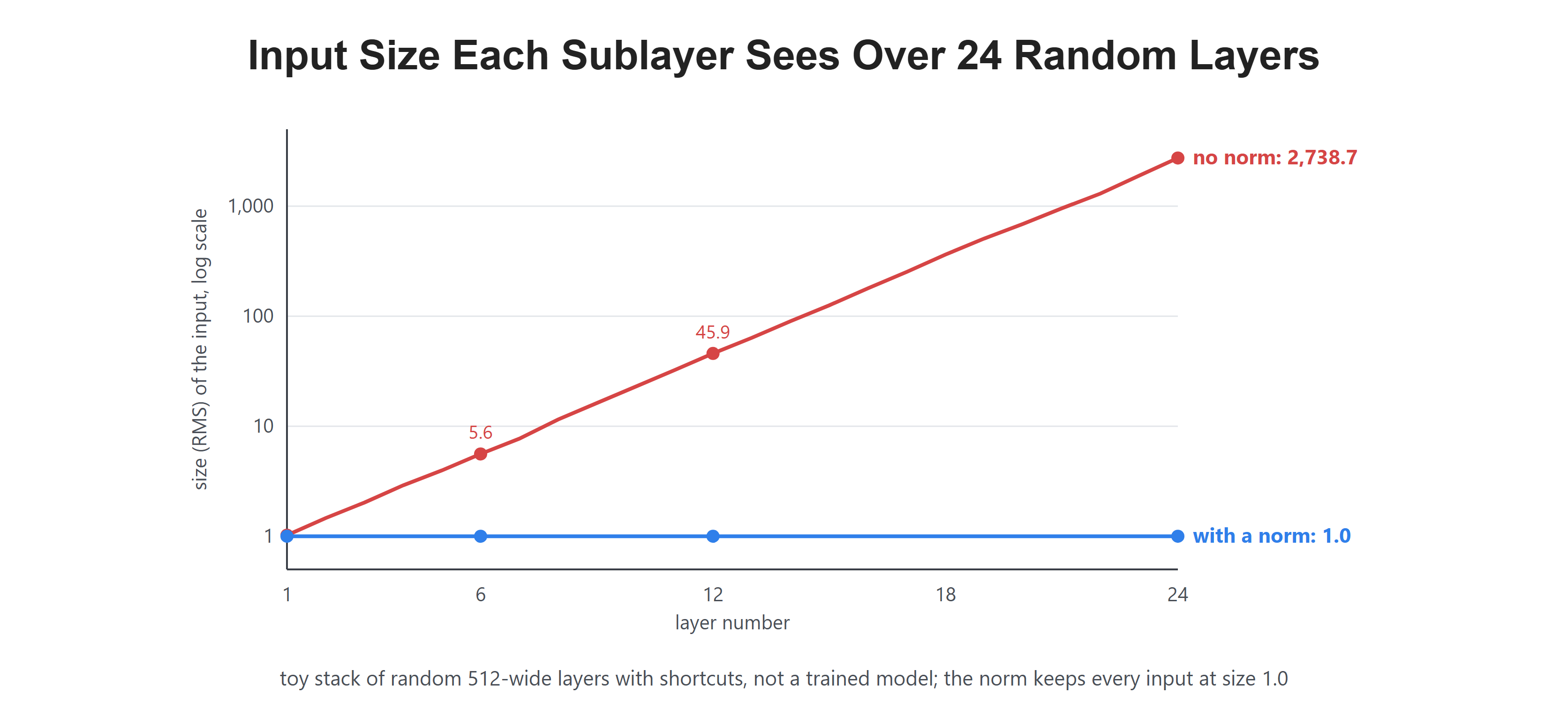
This is a toy with random weights, not a trained model. It only shows how growth piles up when nothing rescales the input.
So, here comes the normalization layer to the rescue. It sits in front of the work, and it hands every layer an input of a steady size.
Which Numbers Does a Norm Look At?
Before we see the formulas, we need to know which numbers get averaged together. Inside an LLM, the data is shaped like a box: sentences, then tokens, then the hidden features of each token.
You may have heard of Batch Norm from image models. It takes one feature and averages it across every token in the batch, from every sentence. That works well for images.
It works poorly for text, for three reasons:
- Sentences have different lengths, so short ones are filled with padding tokens. Unless we mask them out, those fake tokens sneak into the average.
- When a chatbot writes text, it often handles a single sentence at a time. One sentence gives a poor batch average.
- During training, it uses the average of the current batch. At use time, it switches to a saved average, so the model can behave differently.
LLMs pick the other direction. LayerNorm and RMSNorm look at one token at a time, across that token's own features. In simple words, each token is rescaled using only its own numbers. Tokens never share an average, so the length of the sentence and the size of the batch do not matter.
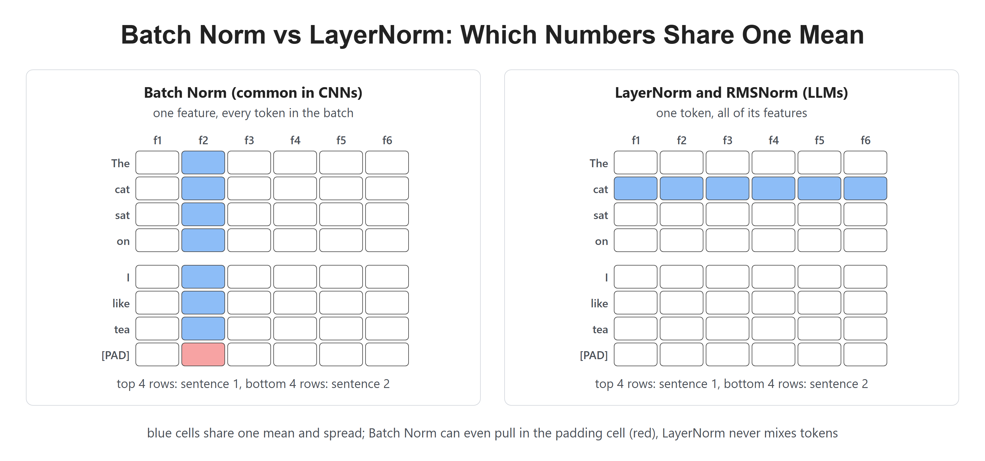
Each blue group shares one average. In LLMs, that group is always one token's own features.
How Does LayerNorm Work?
LayerNorm was introduced by Ba, Kiros and Hinton in 2016. It does two things to a token vector. First, it moves the average of the numbers to 0. Then, it makes their spread equal to 1.
Let's say one token vector is [2, 4, 6, 8].
LayerNorm works on it in four steps:
- Find the mean: (2 + 4 + 6 + 8) / 4 = 5.
- Subtract the mean from every number:
[-3, -1, 1, 3]. - Find the spread. We square each distance (9, 1, 1, 9) and take the mean, which is 5. This is the variance. Its square root, about 2.236, is the standard deviation.
- Divide every centered number by 2.236:
[-1.342, -0.447, 0.447, 1.342].
There is one small detail in step 4. The code adds a tiny number, called epsilon, before the square root. It stops a division by zero when every number in the vector is the same.
Then LayerNorm adds two sets of learned numbers. A gain multiplies each feature, and a bias is added to each feature. Both are trained along with the rest of the model. They start at 1 and 0, so at first they change nothing. Later, they let the model pick its own scale for each feature.
The original Transformer, BERT and GPT-2 all use LayerNorm.
How Does RMSNorm Work?
In 2019, Biao Zhang and Rico Sennrich asked a simple question. Do we really need step 1 and step 2? Their guess was that centering is not needed. Only the rescaling matters. So, they proposed RMSNorm.
RMSNorm skips the mean completely. It divides each number by the RMS of the vector. In simple words, it shrinks or grows the vector to a steady size, and it leaves the average wherever it was.
Let's run the same vector [2, 4, 6, 8] through RMSNorm:
- Square each number: 4, 16, 36, 64.
- Take the mean of the squares: 120 / 4 = 30.
- Take the square root: about 5.477. This is the RMS.
- Divide every number by 5.477:
[0.365, 0.730, 1.095, 1.461].
After that, RMSNorm multiplies by a learned gain, just like LayerNorm. But it has no bias. So it does less work: no mean to find, nothing to subtract, and nothing to add at the end.
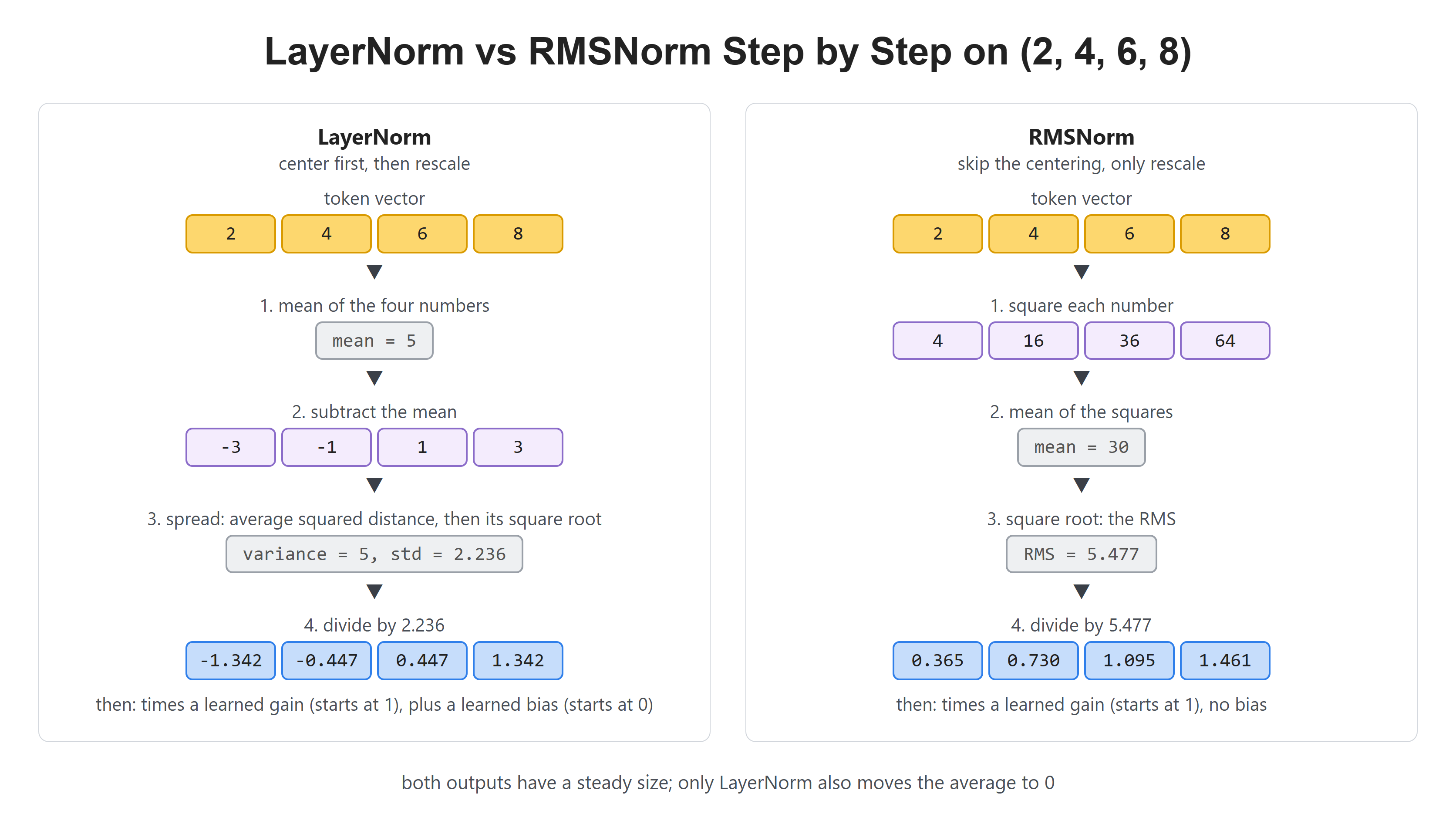
Both outputs end up with a steady size. Only LayerNorm also moves the average to 0.
Llama, Qwen, Mistral, Gemma and DeepSeek all use RMSNorm today.
Let's Check Both Norms in PyTorch
PyTorch ships both layers as nn.LayerNorm and nn.RMSNorm. We create each one for a vector of 4 features and pass in our token. We wrap the call in torch.no_grad() because we are not training, so we do not need PyTorch to track gradients. Let's see the code as below:
import torch
import torch.nn as nn

x = torch.tensor([[2.0, 4.0, 6.0, 8.0]])

layer_norm = nn.LayerNorm(4)
rms_norm = nn.RMSNorm(4)

with torch.no_grad():
    print(layer_norm(x))
print(rms_norm(x))tensor([[-1.3416, -0.4472, 0.4472, 1.3416]])
tensor([[0.3651, 0.7303, 1.0954, 1.4606]])Here, we can see the exact numbers we found by hand. LayerNorm gives values centered on 0. RMSNorm gives values that are all still positive, just smaller.
Now, let's do the same math ourselves, so nothing is hidden. Let's see the code as below:
import torch
x = torch.tensor([[2.0, 4.0, 6.0, 8.0]])

mean = x.mean(dim=-1, keepdim=True)
var = ((x - mean) ** 2).mean(dim=-1, keepdim=True)
print(mean, var)
print((x - mean) / torch.sqrt(var + 1e-5))

rms = torch.sqrt((x ** 2).mean(dim=-1, keepdim=True))
print(rms)
print(x / rms)tensor([[5.]]) tensor([[5.]])
tensor([[-1.3416, -0.4472, 0.4472, 1.3416]])
tensor([[5.4772]])
tensor([[0.3651, 0.7303, 1.0954, 1.4606]])Here, we can see the mean of 5, the variance of 5, and the RMS of 5.4772. Our hand-made results match the PyTorch layers.
Two small choices in this code matter:
dim=-1means "work along the last axis", which is the feature axis. This is what makes the norm look at one token at a time.1e-5is the epsilon. It is the same default thatnn.LayerNormuses.
When Do LayerNorm and RMSNorm Give the Same Answer?
Here is a nice surprise. Let's give both layers a vector whose mean is already 0. We use [-3, -1, 1, 3], the centered version of our token. Let's test it:
import torch
import torch.nn as nn
layer_norm = nn.LayerNorm(4)
rms_norm = nn.RMSNorm(4)

centered = torch.tensor([[-3.0, -1.0, 1.0, 3.0]])

with torch.no_grad():
    print(layer_norm(centered))
print(rms_norm(centered))tensor([[-1.3416, -0.4472, 0.4472, 1.3416]])
tensor([[-1.3416, -0.4472, 0.4472, 1.3416]])Here, we can see two identical rows. When the mean is already 0, subtracting it changes nothing. So the RMS and the standard deviation become the same number, and both layers divide by it.
This is why dropping the mean costs so little in practice. The rescaling does the important job. The centering is a small extra.
The two layers also differ in what they learn. Let's print their learned numbers:
import torch.nn as nn
layer_norm = nn.LayerNorm(4)
rms_norm = nn.RMSNorm(4)

for name, p in layer_norm.named_parameters():
    print("LayerNorm", name, p.data)
for name, p in rms_norm.named_parameters():
print("RMSNorm ", name, p.data)LayerNorm weight tensor([1., 1., 1., 1.])
LayerNorm bias tensor([0., 0., 0., 0.])
RMSNorm weight tensor([1., 1., 1., 1.])Here, we can see that LayerNorm learns a gain (called weight) and a bias. RMSNorm learns only the gain.
Let me tabulate the two norms for your better understanding.
| LayerNorm | RMSNorm | |
|---|---|---|
| Subtracts the mean | yes | no |
| Divides by | standard deviation | RMS |
| Learned numbers per feature | gain and bias | gain only |
| Output average | moved to 0 | left as it was |
| Used in | original Transformer, BERT, GPT-2 | Llama, Qwen, Mistral, Gemma, DeepSeek |
Where Does the Norm Sit in the Block?
Choosing the norm is only half of the story. The other half is where we put it. Let's call the attention or MLP step F. Then there are four common layouts.
Post-norm runs F, adds the shortcut, and then normalizes: x = Norm(x + F(x)). The original Transformer in 2017 used it, and so does BERT. The catch is that the norm sits on the main path, between blocks. In a deep stack, this made early training unstable. These models needed a slow start, called warm-up, where the learning rate begins tiny and grows step by step.
Pre-norm normalizes the input of F and leaves the shortcut untouched: x = x + F(Norm(x)). GPT-2 moved to this layout and added one final norm after the last block. In 2020, Xiong and others showed why it helps. Pre-norm models train well even without the warm-up stage. Llama and Qwen use pre-norm too.
Sandwich puts a norm on both sides of F: x = x + Norm(F(Norm(x))). Gemma 2 and Gemma 3 use it for both attention and the MLP. The second norm tames the size of what F adds back to the stream.
Output norm keeps only the second norm: x = x + Norm(F(x)). OLMo 2 uses this layout, so the input of F is not normalized at all.
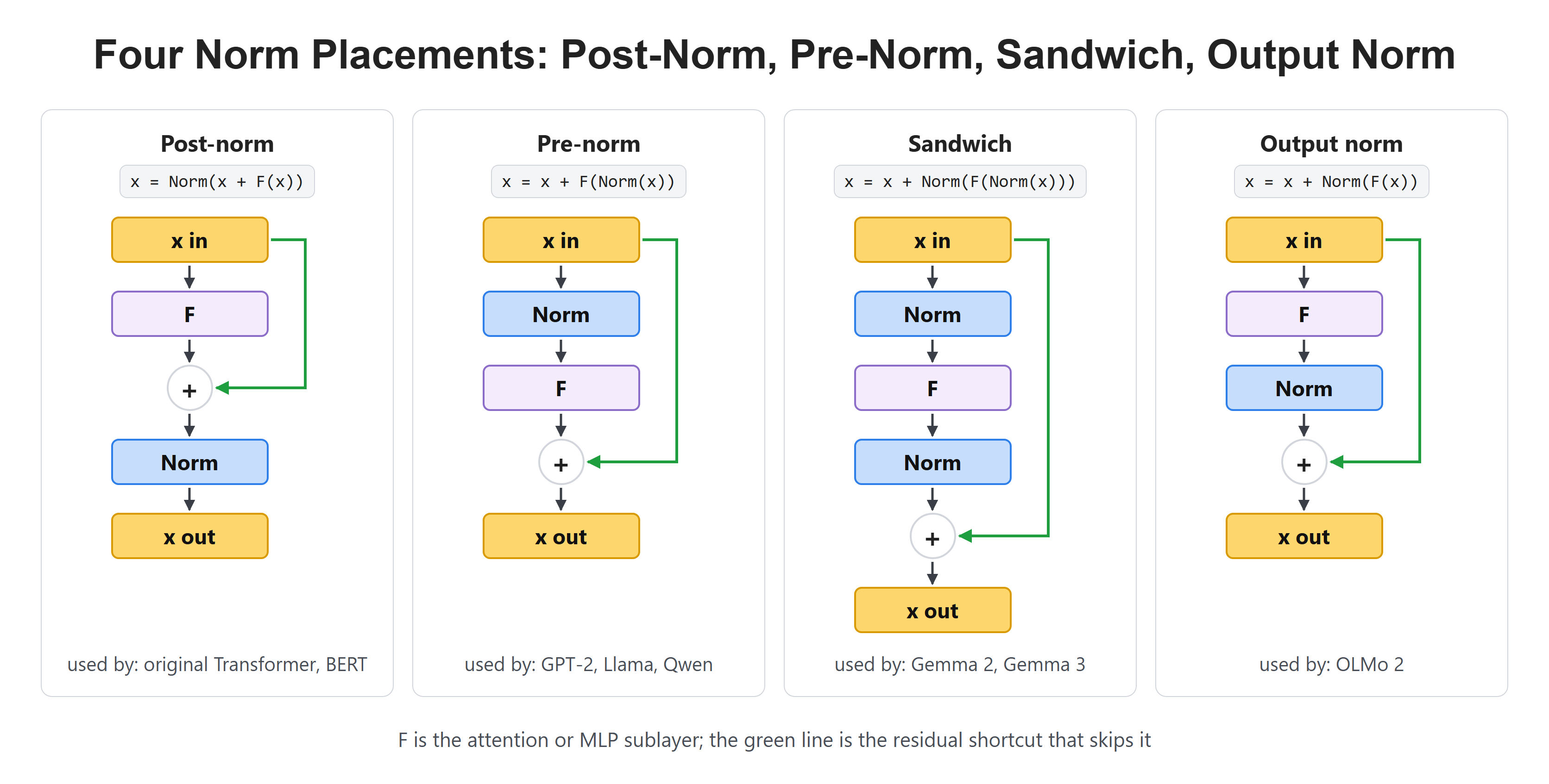
In every layout except post-norm, the green shortcut path never passes through a norm.
Here, we can see the key idea. In pre-norm, sandwich and output norm, the shortcut path stays clean. The residual stream flows from the first block to the last with nothing in its way. That clean path is what makes deep stacks easier to train.
But pre-norm lets the stream itself grow from block to block. So pre-norm models add one final norm after the last block, right before the LM head turns vectors into next-token scores. We saw this final box in the first figure of this lesson.
What Is QK-Norm?
So far, every norm sat outside attention. Newer models add one more pair inside it.
Recall Day 14. An attention score is the dot product of a query and a key. If the queries and keys grow large during training, the scores grow too. Then softmax can put almost all of its weight on one token. When this happens, training can blow up.
QK-Norm rescales each query and each key with an RMSNorm before the dot product. In simple words, it keeps the inputs of the score at a steady size, so the scores cannot drift out of range as easily. The idea comes from Dehghani and others in 2023.
The Qwen3 report says it removes the QKV bias that Qwen2 used and introduces QK-Norm to keep training stable. In the Qwen3 code, q_norm and k_norm work per head, over each head's own features. They run right after the queries and keys are split into heads, and before RoPE adds position.
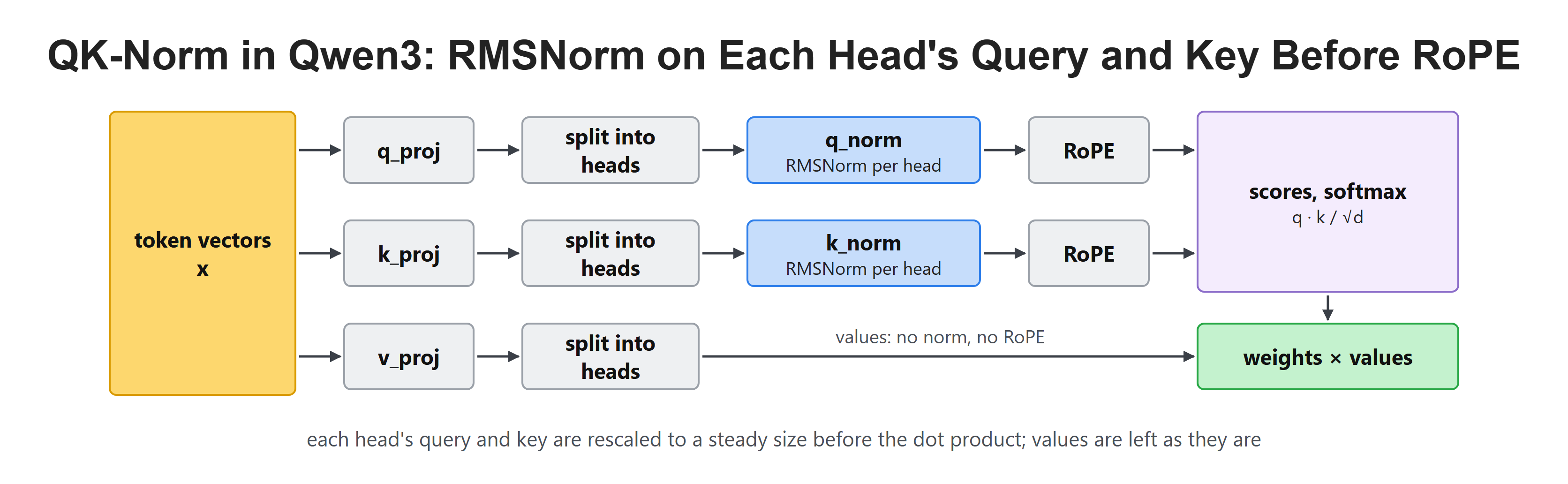
Values skip both the norm and RoPE. Only the two vectors that form the score get rescaled.
Gemma 3 also has q_norm and k_norm. OLMo 2 uses QK-Norm too, but it normalizes all heads of the query together, before the split. The Qwen3 code even has a comment about this difference.
Which Norm Does Each Model Use?
Let me tabulate the models we met in this lesson for your better understanding. We checked every row against its model code in Hugging Face Transformers, except the original Transformer, which comes from the 2017 paper.
| Model | Norm | Placement | QK-Norm |
|---|---|---|---|
| Original Transformer | LayerNorm | post-norm | no |
| BERT | LayerNorm | post-norm | no |
| GPT-2 | LayerNorm | pre-norm + final norm | no |
| Llama | RMSNorm | pre-norm + final norm | no |
| Qwen2.5 | RMSNorm | pre-norm + final norm | no (uses QKV bias) |
| Qwen3 | RMSNorm | pre-norm + final norm | yes, per head |
| Gemma 2 | RMSNorm | sandwich | no |
| Gemma 3 | RMSNorm | sandwich | yes |
| OLMo 2 | RMSNorm | output norm | yes, all heads together |
Here, we can see the trend. The field moved from LayerNorm to RMSNorm, and from post-norm to pre-norm. Newer models then add QK-Norm, a second norm, or both.
Where Else Do Norms Show Up?
Once we know the pattern, we start to see norms in new places:
- DeepSeek V3 squeezes its keys and values into a small vector before it caches them. It puts an RMSNorm on that small vector. We will meet this design in Day 27.
- Qwen 3.8 Flash Next has no
input_layernormand nopost_attention_layernormat all. Its norms moved inside a new kind of shortcut with several lanes. We took it apart in our Qwen 3.8 Flash Next teardown. - For a real RMSNorm traced through every layer of a working model, see our Qwen2.5-0.5B teardown.
Recap
This is how normalization works in LLMs. We started with the problem: without a norm, the input of each layer keeps growing as blocks pile up. We saw why LLMs rescale one token at a time instead of using Batch Norm. Then we worked through LayerNorm, which centers and rescales, and RMSNorm, which only rescales. Finally, we placed the norm in the block. Pre-norm keeps the shortcut path clean, a final norm closes the stack, and QK-Norm keeps the attention scores in range.
On Day 20, we will look at the cost of left-to-right generation and see why a key-value cache makes each new token step cheaper.