"Transformer" is the name of an architecture family, not the name of one single reading rule. The attention calculation from the earlier days appears in several model shapes. The important choice is what information a token may read and what the model must produce at the end.
Two major branches make that difference easy to see. Encoder models such as BERT read a complete input in both directions. Decoder models such as GPT read from left to right and predict the next token.
The overview below places the two families side by side.
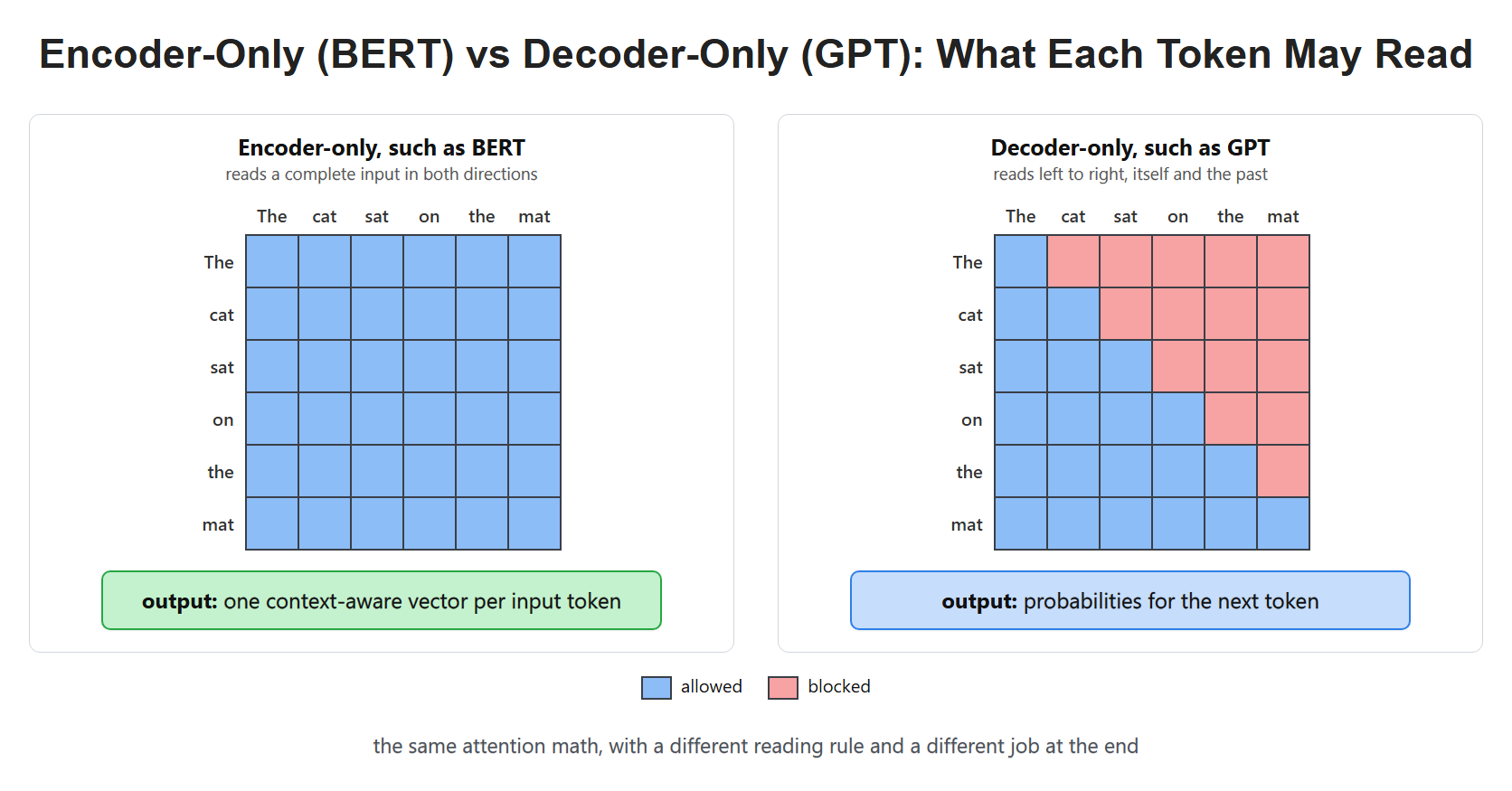
Encoders build representations from a complete input, while decoders grow an output sequence one token at a time.
The Shared Transformer Block Comes First
Before we compare the three families, we need to name the pieces that they repeat. A Transformer is not attention alone. A model starts with token embeddings and position information. Then it sends those vectors through many Transformer blocks. Each block has an attention sublayer, a small neural network called an MLP or feed-forward network, shortcut additions, and normalization.
The attention sublayer lets one token gather useful information from other allowed tokens. The MLP then changes the information at each position on its own. This division is useful: attention decides where to look; the MLP changes what the model can represent after it has looked.
A residual connection, also called a shortcut, adds a sublayer's input back to its output. It gives information a direct path through a deep stack and helps the model learn changes instead of rebuilding every useful feature at every layer.
Layer normalization centers and rescales the features within one token vector, then applies learned scale and offset values. In the common pre-norm layout, normalization happens before attention and before the MLP. It does not mix information between different tokens. It prepares one token's vector for stable computation.
The MLP usually has two learned linear transformations with a non-linear function between them. A non-linearity means the middle step is not just another straight scaling of numbers. Without it, several linear layers could collapse into one linear layer and would not learn richer changes. Many modern models use GELU or SwiGLU for this middle step.
Here is a small pre-norm block written as a learning map. We show the attention step first because it is the part that can read other positions.
x = x + attention(attention_norm(x))attention_norm(x) prepares each token vector. attention(...) gathers allowed context. The x + is the residual connection that keeps the earlier representation available.
The next line works at each token position after attention has mixed context.
x = x + mlp(mlp_norm(x))mlp(...) applies the same learned small network to every token position. It does not choose other tokens to read. The second x + is another residual connection. Repeating the block lets each layer work on features already changed by earlier layers. This does not assign fixed 'simple' or 'abstract' jobs to particular depths.
For a decoder, the attention call uses the causal rule from Day 16. For an encoder, it normally lets all real input tokens see one another. For an encoder-decoder model, the decoder also has a cross-attention sublayer that can read the encoder output.
At the end of a decoder stack, an output head turns the final vector for the newest position into one score, called a logit, for every vocabulary token. Softmax turns those logits into probabilities. The vocabulary score list in the next sections comes from this output head, not from attention directly.
Calculate the Shortcut and Normalization
If the input is and the attention update is , a residual addition gives . The model can learn a small correction while the input keeps a direct path forward. During training, that direct path also contributes to the gradient, the signal describing how a change affects loss. It helps train deep networks but does not guarantee that every gradient stays well behaved.
For layer normalization, use the token vector . Its feature mean is 2, and its mean squared deviation is 1. Subtracting 2 and dividing by approximately 1 produces approximately . The exact denominator is , where a small positive prevents division by zero.
A learned scale and offset then let the model adjust those normalized features. The mean and variance are computed across this token's feature coordinates, not across words or across the batch. Layer normalization does not set a hard upper bound on every resulting number.
The two normalization calls above have separate learned parameters. They are schematic operations, not a standalone runnable model. We name them separately because the attention input and MLP input are different representations.
Pre-Norm Is Not the Original Post-Norm Layout
In a pre-norm block, normalization prepares the sublayer input: . In a post-norm block, the sublayer runs first and normalization follows the addition: .
The original Transformer used post-norm blocks. The short learning map above uses pre-norm to explain a common later arrangement. Neither order should be silently labeled as the only Transformer architecture.
Some later models use RMSNorm, which rescales by the root mean square of the features without subtracting their mean. It serves a related normalization role, but is not the same formula as LayerNorm. When reading an architecture diagram, check both the normalization type and where it sits relative to the shortcut.
What Happens Inside the Feed-Forward Network?
For a tiny example, a feed-forward network can take width 4, expand to width 8, apply an activation, and return to width 4. Expansion creates intermediate features; contraction returns the width required for the next residual addition. The actual expansion ratio is a model choice.
The original Transformer used ReLU, which keeps a positive input and changes a negative input to zero. Without an activation, two linear maps could be replaced by one linear map. The activation lets the network change its behavior depending on the input.
GELU uses a smooth input-dependent change instead of ReLU's sharp cutoff. SwiGLU is a gated design: two projected branches are combined element by element after a smooth activation on one branch. It is not simply another name for a two-matrix ReLU network.
The same feed-forward weights are applied separately at every token position within a layer. Different layers generally have different weights. Tokens can still carry sentence context into that network because the preceding attention already mixed information across positions.
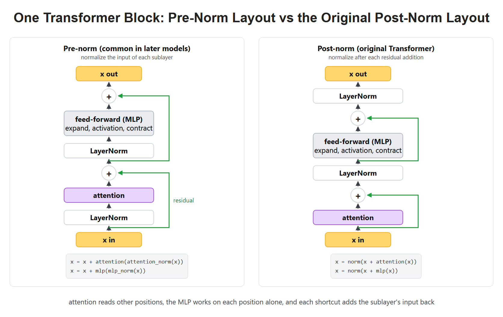
Trace the main path and both shortcut additions. Check whether normalization is before or after each sublayer before interpreting the diagram.
Encoder Models Read the Whole Input
An encoder receives an input sequence that already exists. In a usual encoder self-attention layer, each token may attend to tokens on both its left and its right.
Consider the word bank. In river bank, the word river helps explain the meaning. In bank loan, the word loan helps. A full sentence view gives the token representation access to both clues at the same time.
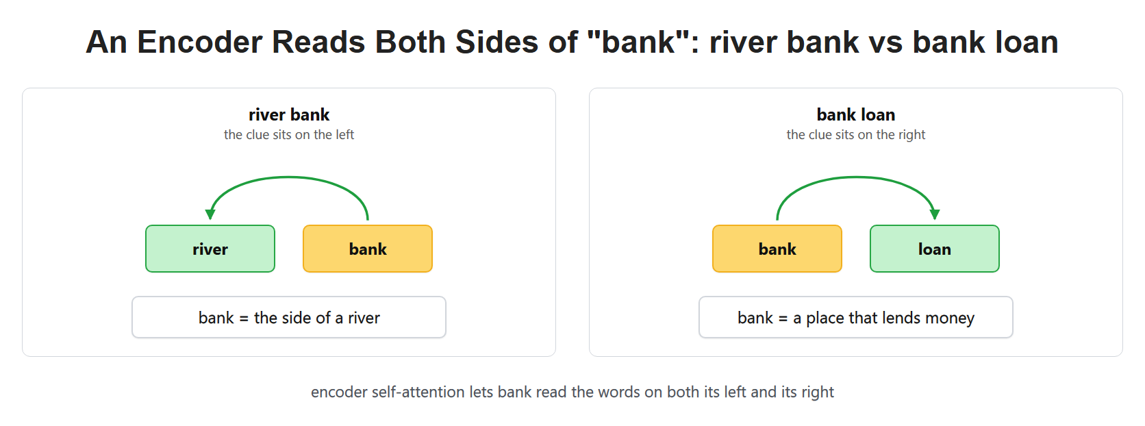
An encoder token can use surrounding context from both earlier and later positions in the input.
This two-sided view makes encoders a natural fit when the input must be understood as a whole. Common examples include sentiment classification, document labels, named-entity tagging, semantic search, and retrieval embeddings.
The Encoder Attention Grid Has No Future Triangle
An encoder still has an attention score grid: queries are compared with keys, softmax makes weights, and values are blended. The usual difference is that the grid does not block its upper triangle for left-to-right causality.
For a normal unpadded input, every token may read every other token. Padding positions can still be masked because they are not real content, but that is a separate issue from hiding future words.
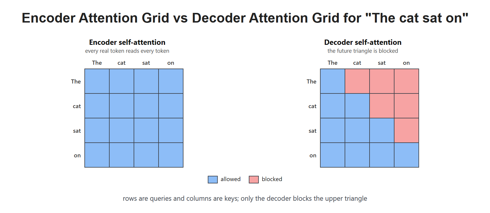
Encoder self-attention normally permits both directions; decoder self-attention blocks the future.
This is why an encoder is called bidirectional in the common BERT-style setup. It is not predicting a sentence from left to right, so it is allowed to use right-side context while building a representation.
BERT Learns by Filling Hidden Pieces
Classic BERT training hides, or masks, selected input tokens and asks the model to predict them from the remaining context. If a sentence says The cat [MASK] on the mat, the word before and the words after the hidden position can help predict sat.
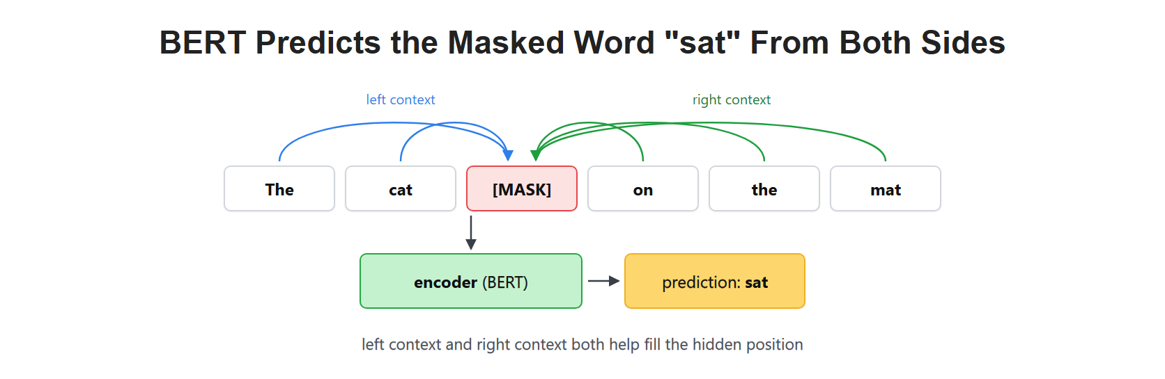
Masked-language training gives the encoder a reason to use left and right context around a hidden input token.
Do not confuse this training mask with the causal mask from Day 16. BERT's [MASK] is a special input token used in the training task. GPT's causal mask is an attention rule that blocks future positions. The two masks solve different problems.
An Encoder Produces a Representation of Existing Text
After its layers, an encoder returns a context-aware vector for every input position. A task head can use one selected vector, a pooled combination of vectors, or all token vectors depending on the job.
For sentiment, a classifier can turn a full-text representation into labels such as positive or negative. For named-entity recognition, a classifier can label every token. For search, an encoder can produce a vector that is compared with other vectors.
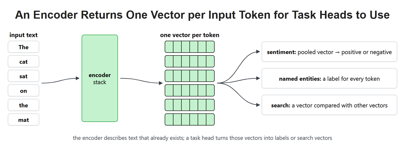
Encoder outputs are useful features for a task that starts from text already supplied by the user or a dataset.
An encoder can be used inside a larger system that writes text, but an encoder-only architecture is not designed to freely continue a prompt token by token.
Decoder Models Predict What Comes Next
A decoder-only model receives a prefix such as The cat and produces a probability for the next token. It must not inspect sat before deciding whether sat is likely. That would let it cheat during training and would not match real text generation.
The causal mask from Day 16 enforces this rule. Every token can read earlier tokens and itself, but not a later token.
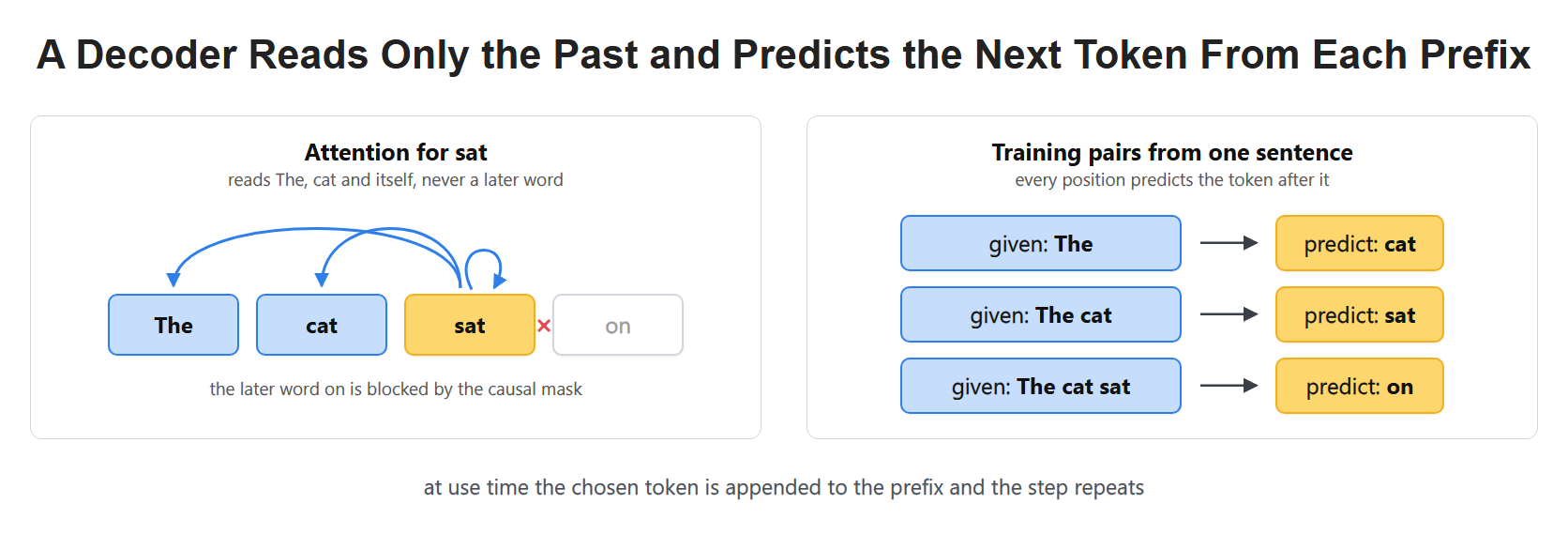
A decoder position can use its generated past, but the future remains blocked.
GPT-style training shifts through a text and asks for the next token at every position. Given The, predict cat. Given The cat, predict sat. Given The cat sat, predict on.
At use time, the model chooses a next token, appends it to the prefix, and repeats. This makes decoder models suitable for chat, continuation, code completion, and other tasks where the output is a new growing sequence.
A Decoder Produces a Growing Sequence
The useful output of a decoder is not just one fixed embedding. Each step supplies a probability distribution over the vocabulary, from which the system selects the next token. The selected token changes the input for the following step.
This is why a decoder can write an answer of a different length from its prompt. The stopping rule decides when to end, often after an end-of-sequence token or a chosen maximum length.
When a Model Uses Both Parts
An encoder-decoder Transformer combines both reading styles. The encoder reads the full source input in both directions. The decoder writes a target sequence with causal self-attention and uses cross-attention to look at encoder output.
Translation is the classic example: encode an English sentence, then decode a French sentence. Summarization and many text-to-text tasks use the same broad pattern.
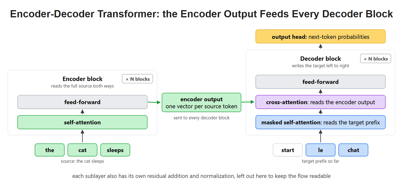
The encoder understands the complete source, and the decoder generates a target while consulting the encoded source.
Follow a translation through the complete system. Source token IDs enter an embedding table and receive source position information. The encoder stack turns them into contextual source vectors. Target input IDs begin with a start marker and the known target prefix, with their own position information.
Inside each decoder block, causal self-attention first reads the target prefix. Cross-attention then reads the encoder's final source vectors. Each attention sublayer has its own residual and normalization arrangement, followed by the feed-forward sublayer and its shortcut. Repeating decoder blocks refines the target representation before the output head produces vocabulary logits.
The encoder output fans out to the cross-attention modules in the decoder layers; it is not consumed and lost after the first decoder block. During training, shifted target labels supply the learning target. During generation, a selected token returns through the target embedding path on the next step.
These are natural starting points, not exclusive task boundaries. A decoder can classify text with an appropriate prompt or head, and retrieval needs suitable training rather than merely choosing any encoder. Architecture defines information flow; training and the output head help determine the task.
The architecture should follow the job, not the model name people mention most often.
| Main job | Natural starting family | Why |
|---|---|---|
| classify or label an existing input | encoder-only | full input context is available |
| generate a continuation or response | decoder-only | output must grow token by token |
| turn one sequence into another | encoder-decoder | decoder can look up the complete source |
Recap
Encoder models such as BERT use bidirectional self-attention to build representations from complete input text. Decoder models such as GPT use causal attention and next-token prediction to generate a sequence from left to right. Encoder-decoder models use both patterns when one sequence must become another.
To teach the distinction back, draw the allowed attention paths for a source sentence and a target prefix. Then add residual connections, normalization, and feed-forward networks. A drawing containing only attention boxes is not a complete Transformer block.
Next, we zoom into one small part of this block, the norm, in LayerNorm vs RMSNorm: How LLMs Normalize Each Token. After that, on Day 20, we will look at the cost of left-to-right generation and see why a key-value cache makes each new token step cheaper.