Yesterday, we saw why a decoder writes one token at a time. That left us with an uncomfortable question. When the model has already read The cat sat, why should it recalculate attention information for The, cat, and sat before predicting the next token?
It should not. A key-value cache, or KV cache, saves the keys and values that earlier tokens produced. At the next step, the model calculates information only for the new token and reads the saved information for the old ones.
The picture below is our map for this lesson. We will use the same small sequence, The cat sat, throughout.
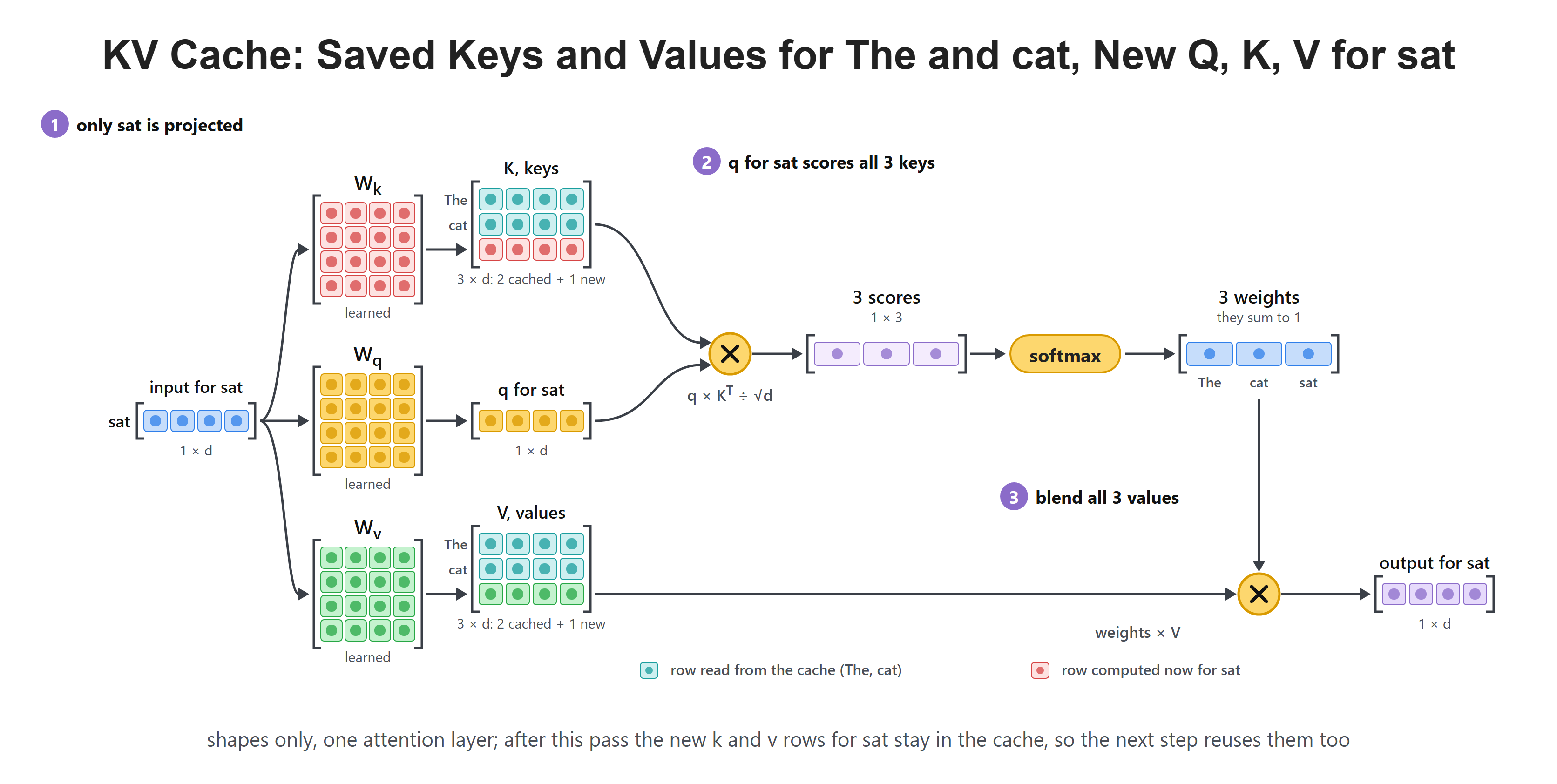
Earlier keys and values stay available while the next token is processed.
First, Recall What Attention Needs
In one self-attention layer, every token is turned into a query, key, and value. A query asks what this position needs. A key says what a token can match. A value carries the information that can be mixed into the answer.
When the model predicts after The cat sat, its new position needs to compare its query with keys for all visible positions. It also needs their values to make the weighted mixture. Those old keys and values are exactly the pieces worth saving.
The old query vectors are not needed again for this next decision. They were useful when their own positions attended earlier in the sequence. For a new token, we need a new query, but the attention table uses old keys and old values.
What Is Stored, and Where?
The cache stores two tensors for every attention layer: one tensor of keys and one tensor of values. It is not one text cache at the top of the model. Layer 1 has its own keys and values. Layer 2 has different keys and values because its input is the output of Layer 1.
This matters because a 24-layer decoder runs attention 24 times. Reusing work in only the first layer would leave most of the repeated work untouched.
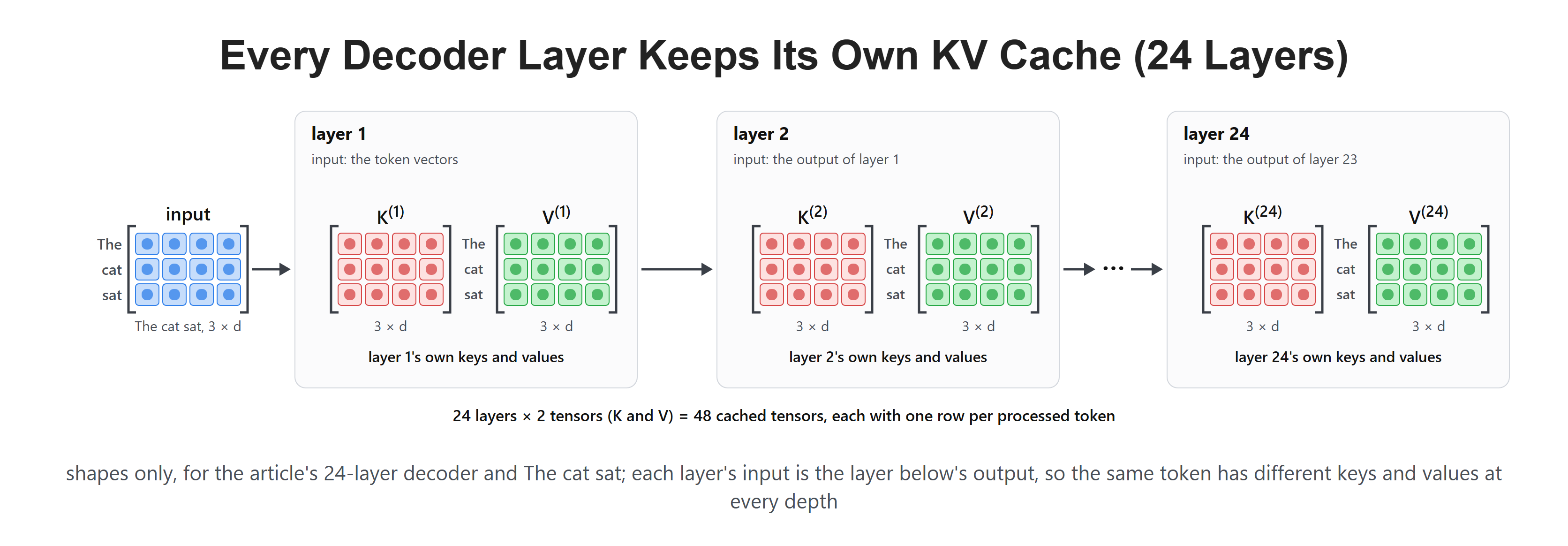
The same token has different key and value vectors at different depths of the model.
The cache also keeps token order. Position 0 is stored before position 1, and so on. On a new step, the layer appends one key and one value at the end of its existing cache.
Why Reuse Is Valid Through the Whole Stack
At layer 1, an earlier token has the same embedding and position as before. Under causal attention it can read only its unchanged prefix. Its output therefore stays the same when a later token is appended.
The same argument applies to layer 2: its earlier input vectors stayed the same, and its mask still blocks later tokens. Repeating this reasoning through the stack shows why earlier keys and values can be reused at every layer.
This assumes unchanged model weights, position handling, prefix tokens, and inference settings, with dropout disabled. Editing an earlier token invalidates the affected cache. An encoder that permits bidirectional attention does not have this append-invariance: a new right-hand token can change earlier outputs.
A cache entry is also not a copy of a word embedding. At higher layers it comes from a context-dependent hidden state, which explains why two requests containing the same word can need different cache entries.
The Prompt Is Processed Once
Suppose the prompt is The cat. Before the model can suggest sat, it processes both prompt tokens. Each layer produces keys and values for The and cat. We save them as the initial cache.
This first pass is called prefill. It fills the cache from the already-known prompt. The model still does normal attention while it reads the prompt, because all prompt positions need their own outputs.
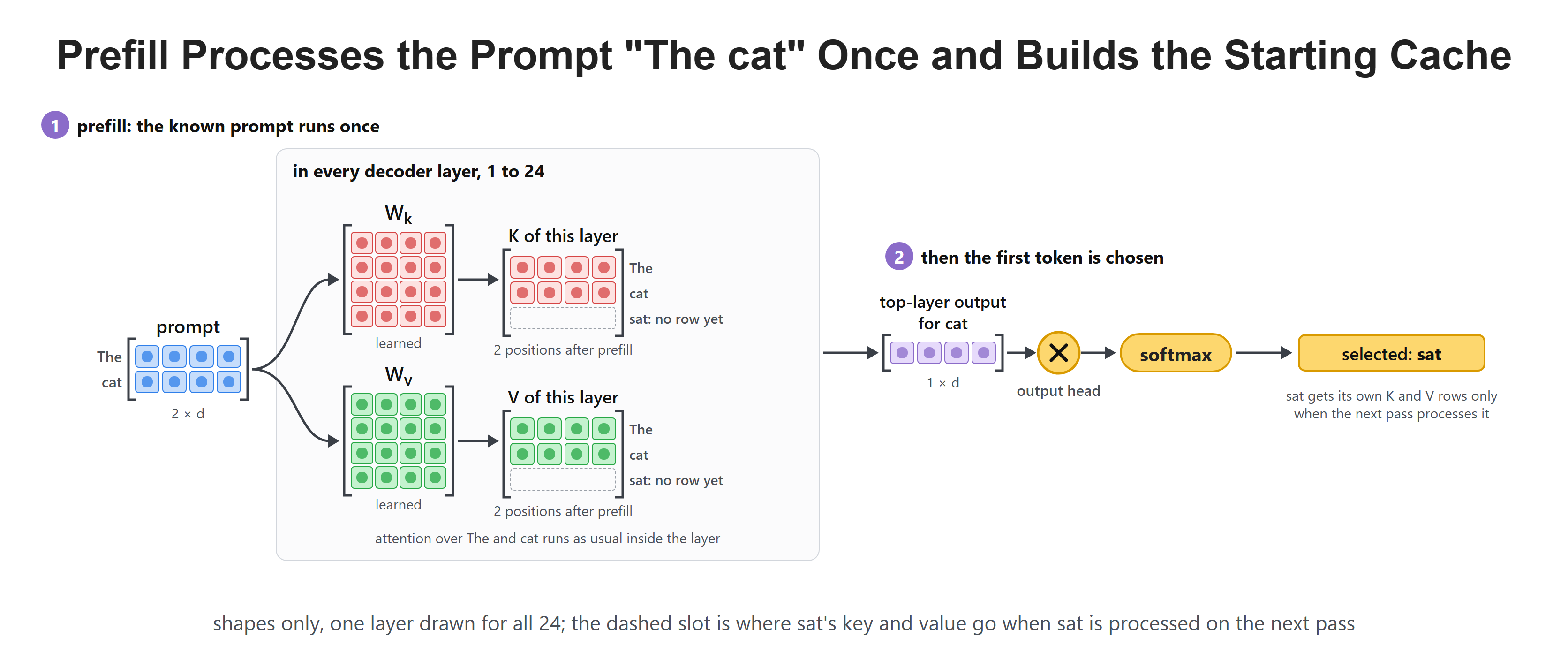
The known prompt builds the starting cache once.
After prefill, the model chooses a next token. Let us say it chooses sat. That token is now fixed input, not a guess we can ignore. Its key and value must join the cache before the next prediction.
One Cached Decoding Step
At the next step, the first layer receives the representation for sat, rather than the whole three-token sequence. Later layers receive that same position's updated hidden state from the layer below, not its raw token embedding. It makes a new query, key, and value for sat. The new query compares with the saved keys for The and cat plus its own new key. Then it uses the matching weights on the saved values plus its own new value.
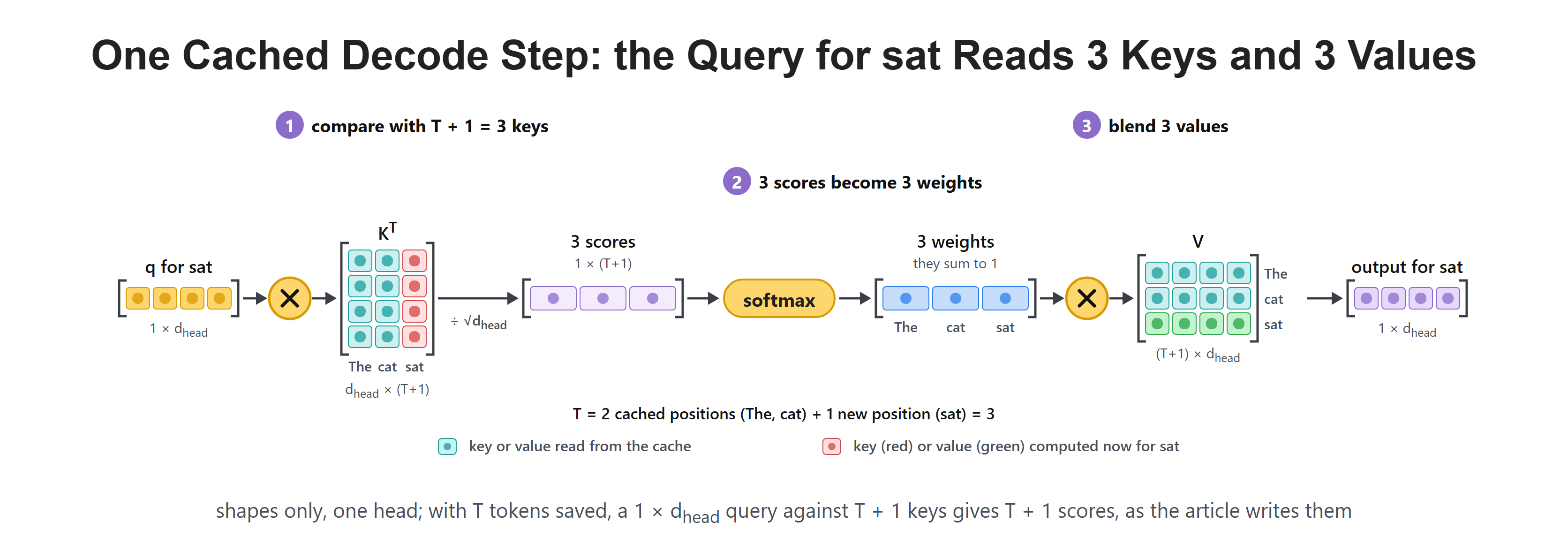
Only the newest position creates fresh Q, K, and V vectors.
Written in shapes, a new query has one position while the cache has all earlier positions. If T tokens are already saved, the new query has shape 1 x d_head; the keys have shape T+1 x d_head. Their dot products give T+1 attention scores.
The model does not need to rebuild key vectors for the first T tokens. Their text, positions, and earlier context have not changed.
Follow the Timing Without Skipping a Pass
| Work just completed | Processed positions in each layer's cache | Newly selected output |
|---|---|---|
Prefill The cat |
The, cat | sat |
Process sat |
The, cat, sat | on |
Process on |
The, cat, sat, on | the |
Selecting sat does not calculate its projections. Those require its hidden state to pass through the layers. This distinction matters when counting cache positions, designing a stopping rule, or writing a diagram of the loop.
The newest query at the second row reads three positions, including its own newly computed key. It is not a query for the still-unknown on token. It is the query derived from sat that helps the model predict what follows.
The Cache Grows One Token at a Time
After sat, imagine the model chooses on, then the. Each chosen token contributes one more key and one more value in every layer when it is processed on the next forward pass. A cache that began with two prompt positions becomes length three, then four, then five.
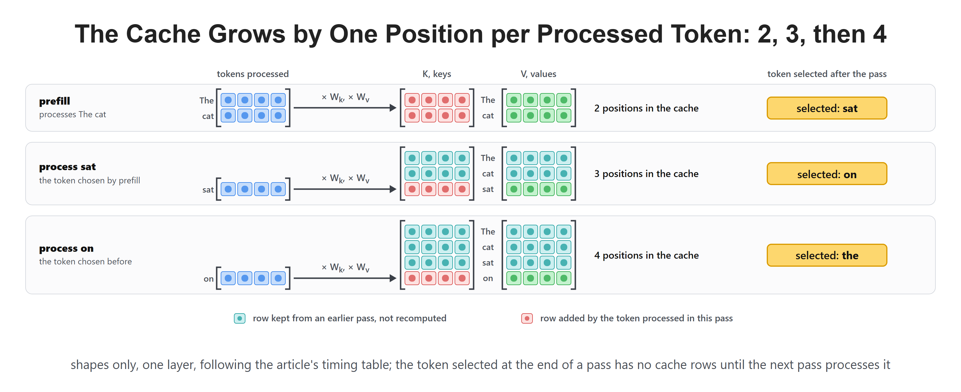
Each processed input token adds a position; the token selected at the end of that pass has not been processed yet.
This is why we call it a cache rather than a shortcut in the attention formula. It records results that can be reused later. It does not change the meaning of causal attention.
What Work Does It Remove?
Without caching, a step after The cat sat on could run the entire prefix through every layer again. That repeats key and value projections for The, cat, sat, and on. With caching, the layer projects only the new token.
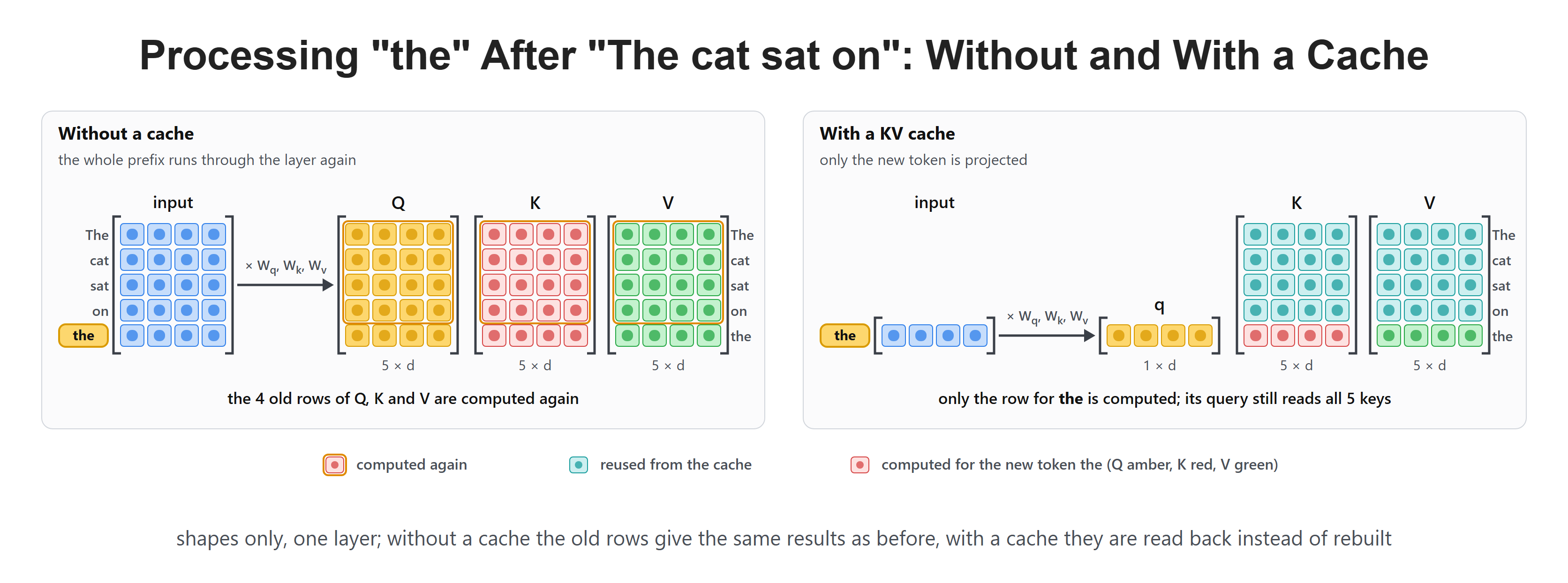
Teal rows are reused from the cache; only the new token, "the", needs new projections.
There is still a comparison between the newest query and the old keys. The cache avoids rebuilding old representations. It does not mean the new token can forget the earlier context.
What the Cache Does Not Solve
The cache cannot predict on before the model has chosen sat. The selected token changes the input, so the next step still waits for the current step. This is the main reason generation has lower parallelism than training.
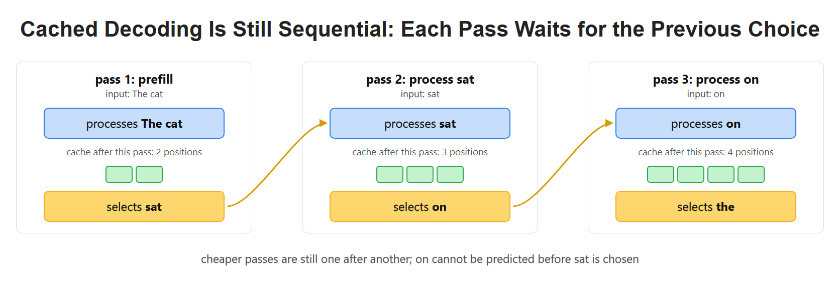
The arrows still move left to right, one selected token at a time.
The cache also consumes memory. A longer prompt, a longer answer, or more requests means more saved keys and values. Tomorrow we will calculate that memory instead of treating it as a vague problem.
A Small Array Model of the Append
We can show the append without installing a full model. NumPy lets us represent one head with two cached positions and two features per position.
import numpy as npThe old rows correspond to The and cat. The new row stands for the projected key of the now-processed sat. Values have the same position count but different contents.
old_keys = np.array([[1., 0.], [0., 1.]])
new_key = np.array([[1., 1.]])
old_values = np.array([[2., 0.], [0., 2.]])
new_value = np.array([[1., 3.]])
keys = np.concatenate([old_keys, new_key], axis=0)
values = np.concatenate([old_values, new_value], axis=0)
assert keys.shape == values.shape == (3, 2)
Axis 0 is the position axis in these two-dimensional arrays. In the common four-dimensional layout [batch, heads, positions, features], the position axis is -2 instead. The axis number follows the layout, not a universal cache rule.
These are invented projections. They demonstrate storage order, not a complete trained attention calculation. Later queries can read all three K/V rows, while the earlier queries need not be saved.
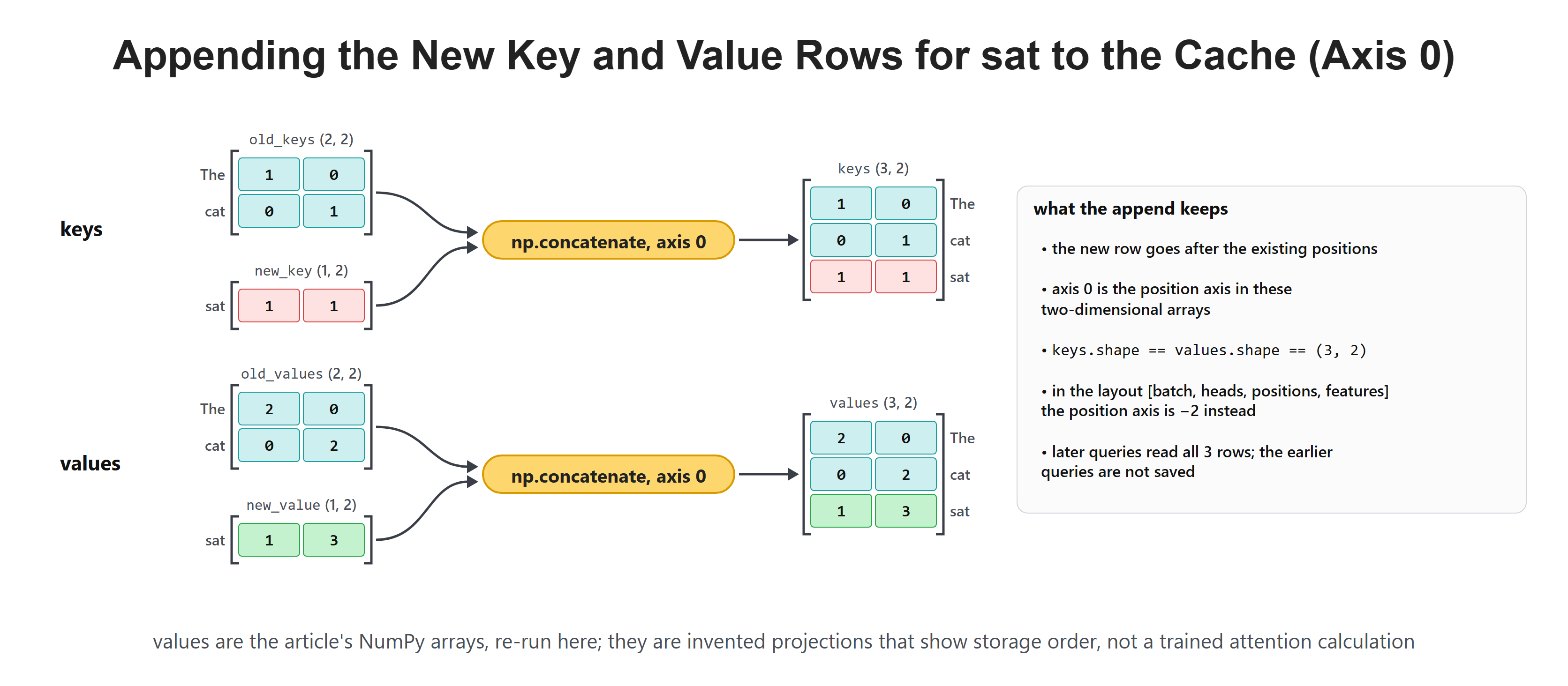
The new key and value are appended after the existing sequence positions.
Real inference engines avoid repeatedly allocating a larger tensor for every small append. Later lessons will show storage methods that make this practical for many requests.
Recap
This is how a KV cache speeds up autoregressive decoding. Every attention layer saves the keys and values for tokens it has already processed. A new token makes fresh Q, K, and V vectors, then its query reads the saved old keys and values plus its own new entry.
The cache removes repeated work on the old prefix. It does not remove the left-to-right dependency, and it grows with every token. Day 22 turns that growth into a VRAM calculation.