In Day 16, we used a causal mask so a word could look left but not right. That rule is easy to understand when a complete training sentence is already on the page. Generating text is different. After the model writes one new token, that token becomes part of the input for the next decision.
We call this autoregressive generation. The model creates a sequence by repeatedly predicting one next token from the tokens already available. A token can be a whole word, part of a word, or punctuation.
The first diagram gives us the big picture: the decoder grows a sentence one token at a time.
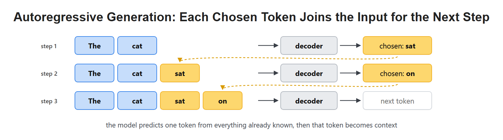
The answer after each step becomes part of the context for the following step.
:::note Autoregressive does not mean that the model copies its last word. It means that the model uses all earlier tokens, including tokens it generated itself, to predict the next token. :::
Why Can the Model Not Write the Whole Answer at Once?
Suppose the prompt is The cat. The model may choose sat as its next token. Only after that choice does the next input become The cat sat. Now it can estimate whether on, near, quietly, or something else should come next.
The token after sat was not hidden somewhere in the prompt. It did not exist as an input token until the model made the earlier choice. This is the dependency that makes normal decoding step by step.
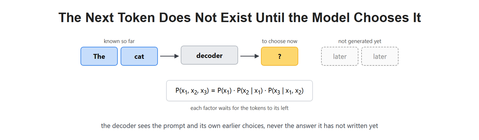
At each step, the decoder sees the prompt plus the tokens it has already chosen, not the future answer.
We can write the same idea with probabilities. For a short three-token output, the probability of the full sequence is:
Read the expression from left to right. First, the model chooses . Next, it chooses while knowing . Finally, it chooses while knowing both earlier choices. The vertical bar means "given that we already know".
This is not a limitation of a slow computer. It is part of the task. If the first chosen token changes, the probability list for the next token can also change.
One Choice Changes the Next Probability List
Imagine the model has written I went to the. If it now chooses bank, the next token might be to, and, or for. If it chooses beach, the next token might be with, yesterday, or a word about water. One selected token changes the context that attention reads on the next pass.
Before the decoder can choose, its final Transformer block produces one vector for the newest position. An output head is a learned final linear layer that turns this vector into one score for every vocabulary token. These raw scores are called logits. A logit is not yet a probability. Softmax changes the full logit list into probabilities that add to 1.
During training, the target is simply the next token shifted one place left. For The cat sat, the visible input at one position is The and the target is cat; at the next position the visible input is The cat and the target is sat. Cross-entropy loss raises the cost when the correct target receives too little probability. This gives the model a clear signal for changing its weights.
At use time, we do not supply that correct next token. A decoding rule picks from the output-head probabilities. Greedy decoding picks the highest probability. Sampling can pick from several likely choices. Either way, the selected token must be added to the input before the next prediction.
That repeated cycle is why even a short answer takes several decoding steps.
From One Hidden Vector to One Token
Suppose the final hidden vector is and our teaching vocabulary has only three tokens: sat, slept, and ran. Let the vocabulary projection have rows and . Multiplying the hidden vector by this two-by-three matrix gives logits .
Softmax turns these logits into approximately . Greedy decoding chooses slept because its probability is greatest. These numbers are invented, not a trained model's predictions.
We can reproduce that output-head step with a small NumPy calculation. It illustrates only the final projection and selection, not the full decoder.
import numpy as npThe three columns correspond to the vocabulary in the same order as the token list. Changing that order without changing the matrix would attach scores to the wrong words.
hidden = np.array([1., 2.])
vocabulary = ["sat", "slept", "ran"]
output_matrix = np.array([[1., 0., -1.], [0., 1., 0.]])
logits = hidden @ output_matrix
exp_logits = np.exp(logits - logits.max())
probabilities = exp_logits / exp_logits.sum()
chosen = vocabulary[int(np.argmax(probabilities))]
Greedy selection finds the best next token under this distribution. It does not search all possible complete sentences to find the most likely sequence. Sampling instead draws a token according to a distribution. Temperature divides logits before softmax: a higher positive temperature flattens the distribution, while a lower one sharpens it.
Top-k sampling retains a chosen number of highest-scoring candidates. Top-p sampling retains the smallest leading set whose cumulative probability reaches a chosen threshold. These rules control selection, not the Transformer weights or the causal mask.
Training Looks Faster for a Different Reason
This can feel confusing because the same decoder predicts every position in a training sentence at the same time. For example, with The cat sat, training can ask for predictions after The, after The cat, and after The cat sat in one matrix operation.
The causal mask still blocks future words. The position for cat cannot read sat. But the teacher has already supplied the complete training sentence, so all those left-side contexts are known before the forward pass begins.
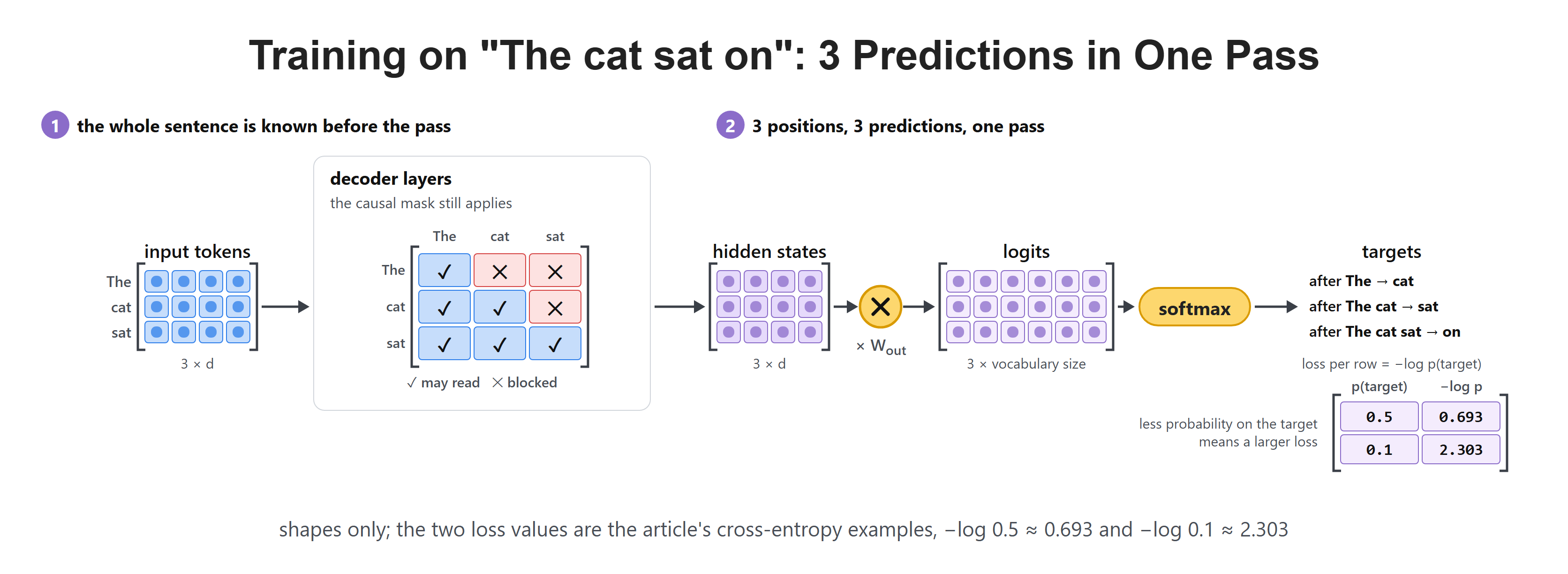
Training has the complete example in advance; generation creates its own future input one token at a time.
During generation, the model does not receive the correct future answer from a teacher. It must live with the token it selected, add it to the prompt, and continue. This difference is often called teacher forcing during training versus autoregressive decoding during use.
Teacher forcing means training uses the dataset's actual earlier tokens, even if the model would have chosen different ones. Cross-entropy for a target token is : a target probability of 0.5 costs about 0.693, while 0.1 costs about 2.303. Assigning less probability to the correct target gives a larger loss.
Training then computes gradients and updates learned weights. Ordinary inference does neither: it keeps weights fixed and updates only the input sequence and temporary request state, including the cache. Predicting many training positions in one pass does not mean an entire training run costs less than generating an answer. It means the known positions provide more work that can be done at the same time.
Where Does the Repeated Work Come From?
At the first step, each attention layer creates keys and values for the prompt tokens. At the next step, the old tokens have not changed. Without a special shortcut, a new full forward pass would calculate their keys and values again, even though those results are the same.
For The cat, then The cat sat, then The cat sat on, the work for The would be repeated at every step. As the answer gets longer, this repeated work becomes expensive.
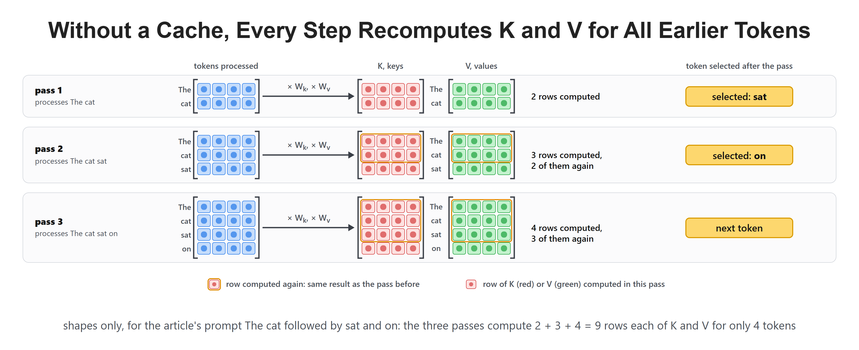
Recomputing keys and values for unchanged earlier tokens wastes work at every new step.
Notice the exact thing we can reuse. A token's old key and value depend on that token and the earlier context it was allowed to read. Once generated text is fixed, those earlier key and value vectors do not need to change. The new token needs a new query, key, and value, but the old ones can stay.
The Key-Value Cache Keeps Earlier Work
A key-value cache, often shortened to KV cache, stores the key and value vectors from past tokens for every attention layer. When the next token arrives, the layer calculates only the new token's query, key, and value. Its query then compares with the stored old keys and the new key together.
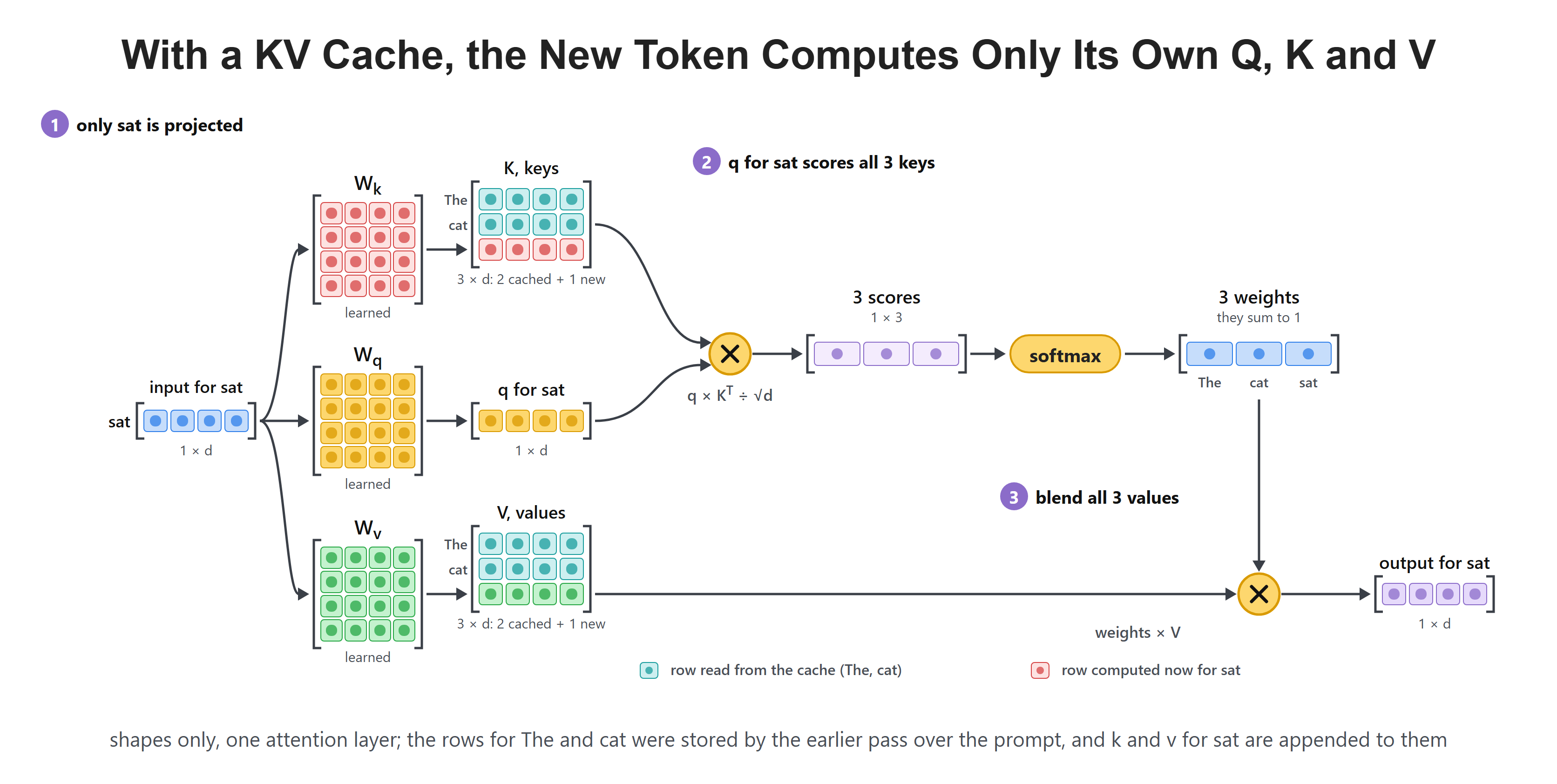
At a new step, the decoder appends one key and one value instead of rebuilding all earlier ones.
This is a cache at every layer, not a single cache at the end of the model. Layer 1 has its own old keys and values. Layer 2 has a different set. The same idea repeats through the stack because every layer performs attention.
The cache grows by one position when a selected token is processed through the model on the following forward pass, not at the instant that token is selected. For a batch of requests, each request needs its own history because the prompts and generated answers are different.
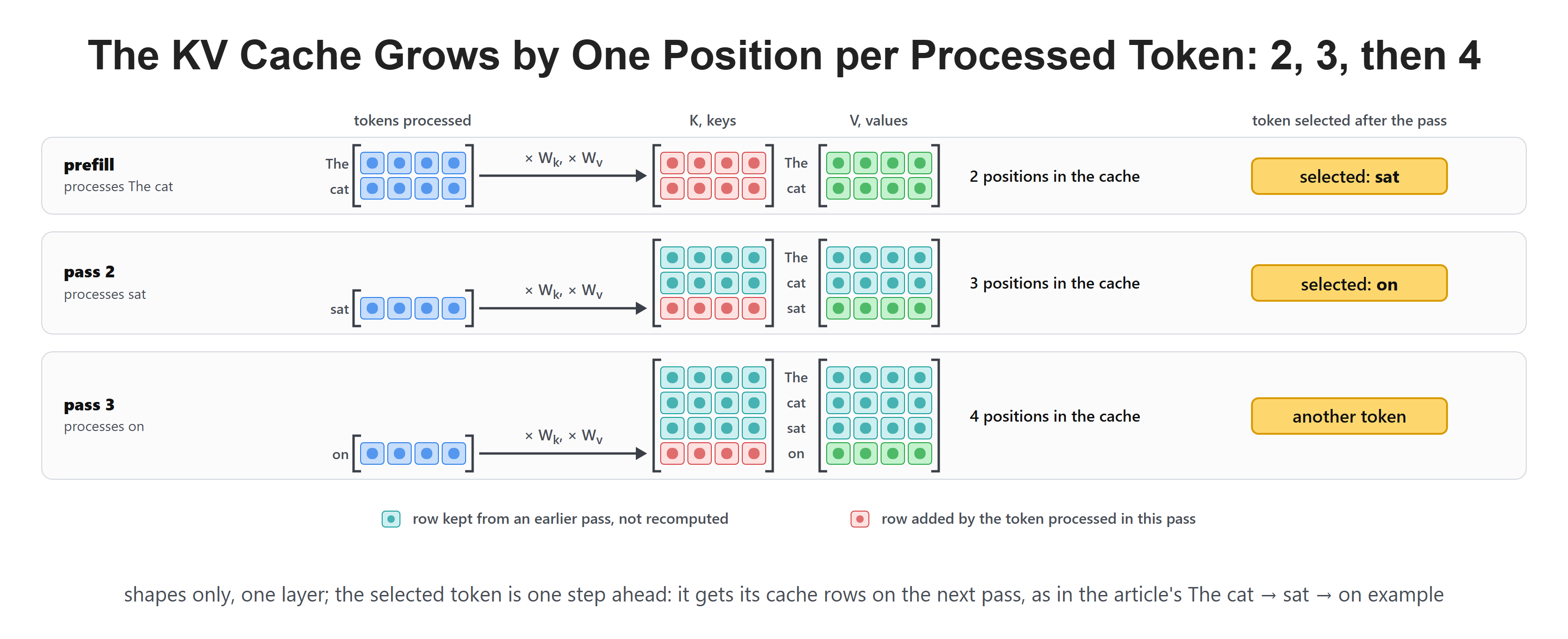
A generated token gains cache entries when it is processed as the next input.
Track the exact boundary with a two-token prompt. Prefill processes The cat, leaves two cache positions, and selects sat. The next pass processes sat, leaves three cache positions, and selects on. A further pass processes on, leaves four positions, and selects another token.
The selected output is one step ahead of the processed cache at these boundaries. If an end token stops the answer immediately, that final selected token need not make another trip through the model.
What the Cache Cannot Fix
The KV cache avoids recalculating old keys and values. It does not remove the left-to-right dependency. The model still needs the chosen token from step 4 before it can form the input for step 5.
Think of it as keeping your earlier arithmetic on the page. You save time because you do not redo it, but you still cannot answer the next question until you know the result of the current one.
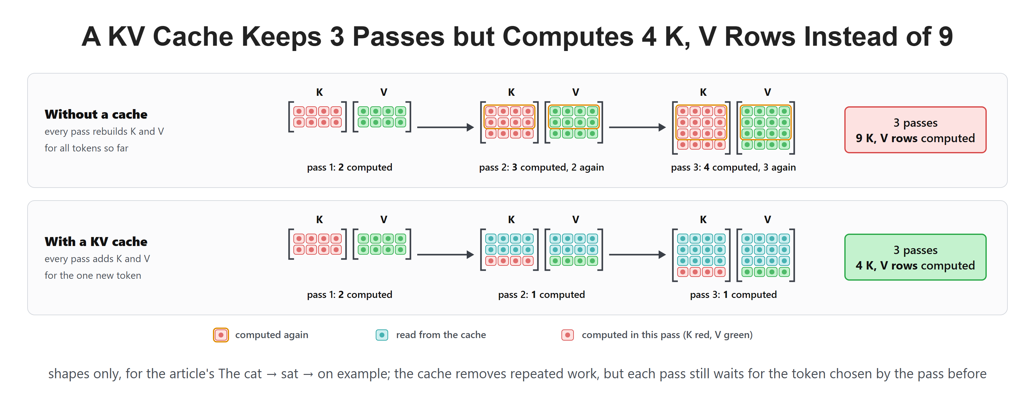
Caching makes each step cheaper, but the decoder still produces one new token per step.
The cache also uses memory. A longer prompt or a longer generated answer means more saved key and value vectors. This is why serving long contexts needs both enough memory and careful cache management.
The Complete Decoding Loop
We can now describe one generation step precisely:
- Process the known prompt once, retaining its layer-by-layer keys and values. This is prefill.
- Use the final prompt position's output to choose the first generated token.
- Append that selected token to the text. It does not yet have its own cache entries.
- If generation should continue, process that token through every decoder layer. Each layer adds its new K and V and reads the allowed cache.
- Use the resulting final hidden state to choose the following token.
- Repeat from step 3 until an end token or length limit stops generation.
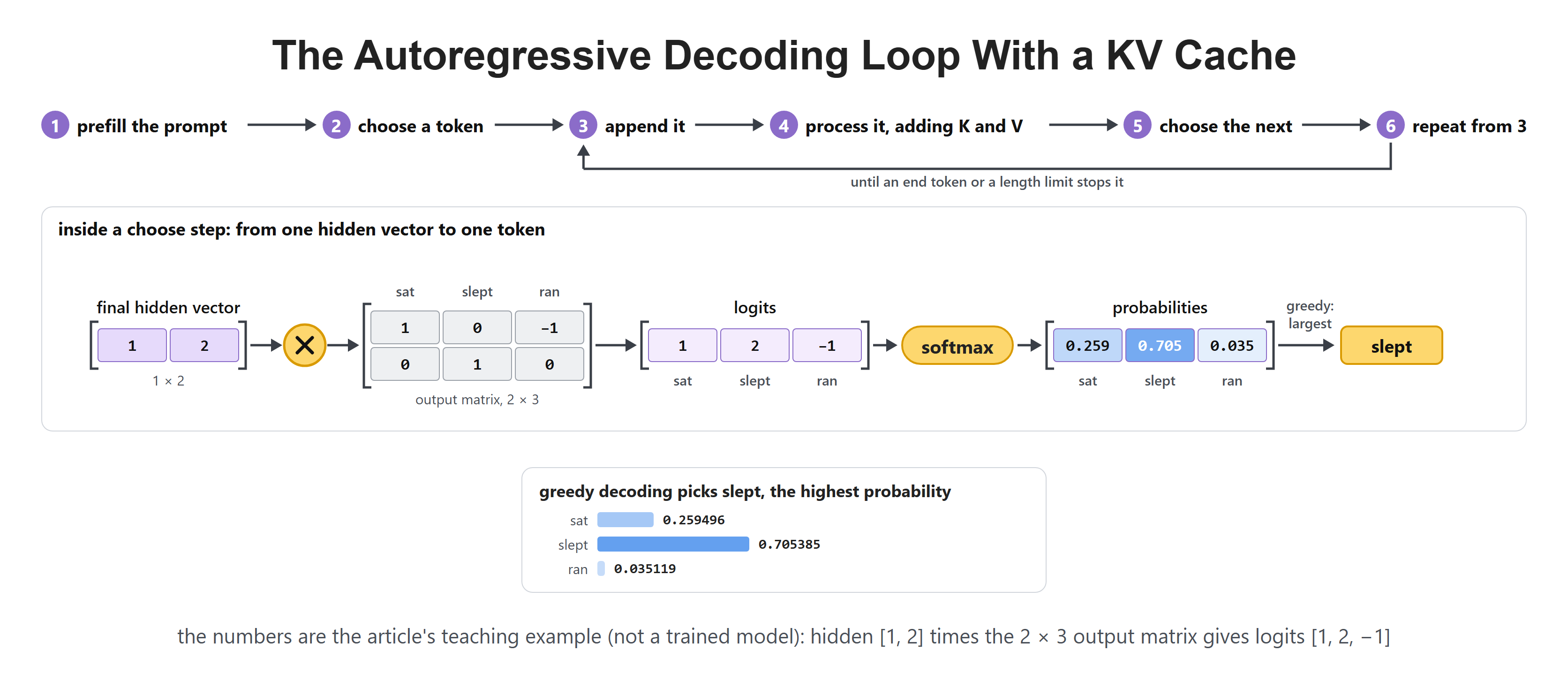
The loop repeats until a stopping rule ends the answer.
Recap
Autoregressive generation means predicting one token from the tokens already known, then using that choice as context for the next token. Training can predict many positions together because the full training example is already given. Generation cannot do that because later tokens depend on earlier choices.
A key-value cache stores attention keys and values from past tokens at every decoder layer. It makes each new step cheaper by avoiding repeated work. It does not make all future tokens available at once, so text generation remains a step-by-step process.