What is CNN

This Notebook demonstrates training a simple Convolutional Neural Network (CNN) to classify CIFAR images.

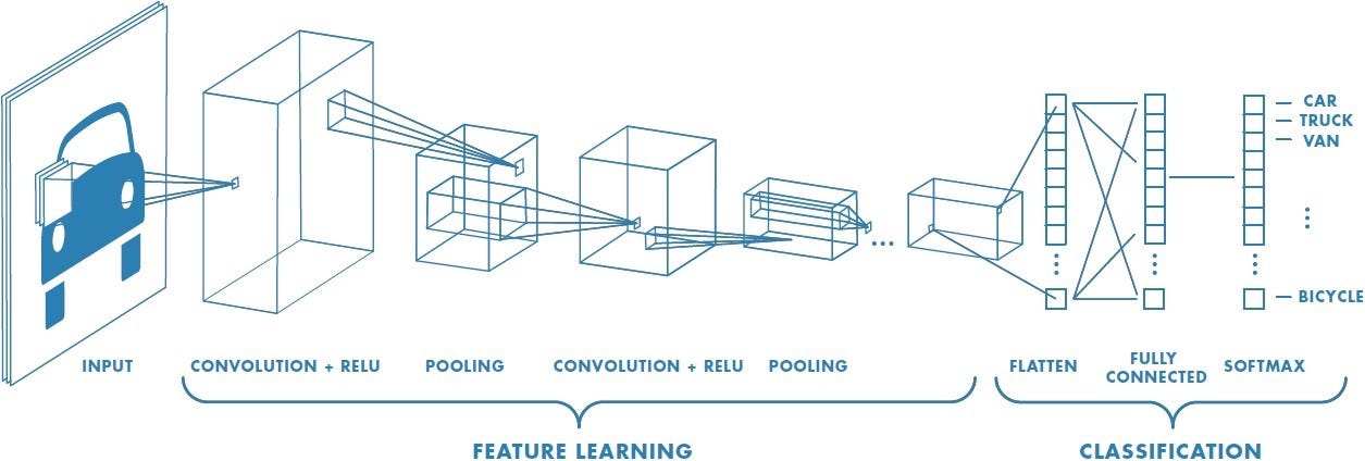
Convolutional Neural Networks (ConvNets or CNNs) are a category of Neural Networks that have proven very effective in areas such as image recognition and classification. Unlike traditional multilayer perceptron architectures, it uses two operations called convolution and pooling to reduce an image into its essential features, and uses those features to understand and classify the image.

Important Terms of CNN

Convolution Layer

Convolution is the first layer to extract features from an input image. Convolution preserves the relationship between pixels by learning image features using small squares of input data. It is a mathematical operation that takes two inputs such as image matrix and a filter or kernel.Then the convolution of image matrix multiplies with filter matrix which is called Feature Map.

Convolution of an image with different filters can perform operations such as edge detection, blur and sharpen by applying filters.

Activation Function

Since convolution is a linear operation, and images are far from linear, nonlinearity layers are often placed directly after the convolution layer to introduce nonlinearity to the activation map.

There are several types of nonlinear operations, the popular ones being:

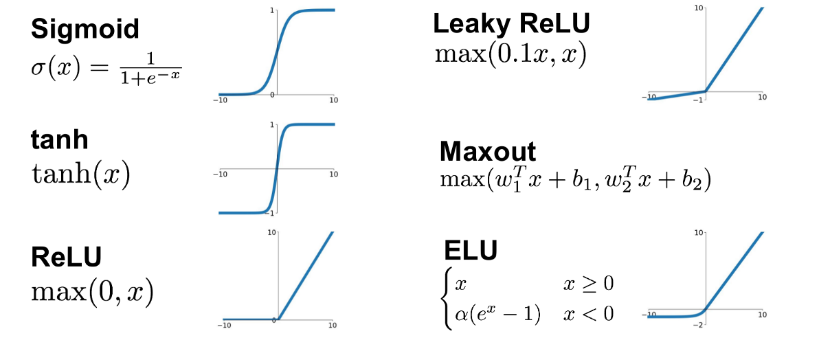
Sigmoid: The sigmoid nonlinearity has the mathematical form f(x) = 1 / 1 + exp(-x). It takes a real-valued number and squeezes it into a range between 0 and 1. Sigmoid suffers a vanishing gradient problem, which is a phenomenon when a local gradient becomes very small and backpropagation leads to killing of the gradient.

Tanh: Tanh squashes a real-valued number to the range [-1, 1]. Like sigmoid, the activation saturates, but unlike the sigmoid neurons, its output is zero-centered.

ReLU: The Rectified Linear Unit (ReLU) computes the function ƒ(κ)=max (0,κ). In other words, the activation is simply threshold at zero. In comparison to sigmoid and tanh, ReLU is more reliable and accelerates the convergence by six times.

Leaky ReL:Leaky ReLU function is nothing but an improved version of the ReLU function. Leaky ReLU is defined to address this problem. Instead of defining the Relu function as 0 for negative values of x, we define it as an extremely small linear component of x.

Maxout:The Maxout activation is a generalization of the ReLU and the leaky ReLU functions. It is a learnable activation function.

ELU:Exponential Linear Unit or ELU for short is also a variant of Rectiufied Linear Unit (ReLU) that modifies the slope of the negative part of the function.Unlike the leaky relu and parametric ReLU functions, instead of a straight line, ELU uses a log curve for defning the negatice values.

Filter | Kernel Size | Number of Filters

Convolution is using a kernel to extract certain features from an input image.A kernel is a matrix, which is slideacross the image and multiplied with the input such that the output is enhanced in a certain desirable manner.

Before we dive into it, a kernel is a matrix of weights which are multiplied with the input to extract relevant features. The dimensions of the kernel matrix is how the convolution gets it’s name. For example, in 2D convolutions, the kernel matrix is a 2D matrix.

A filter however is a concatenation of multiple kernels, each kernel assigned to a particular channel of the input. Filters are always one dimension more than the kernels. For example, in 2D convolutions, filters are 3D matrices. So for a CNN layer with kernel dimensions hw and input channels k, the filter dimensions are kh*w.

A common convolution layer actually consist of multiple such filters.

Stride Size

Stride is the number of pixels shifts over the input matrix. When the stride is 1 then we move the filters to 1 pixel at a time. When the stride is 2 then we move the filters to 2 pixels at a time and so on. The below figure shows convolution would work with a stride of 1.

Padding

padding means giving additional pixels at the boundary of the data.Sometimes filter does not perfectly fit the input image then we will be using padding.

We have two options:

• Pad the picture with zeros (zero-padding) so that it fits
• Drop the part of the image where the filter did not fit. This is called valid padding which keeps only valid part of the image.

Pooling Layer

A pooling layer is a new layer added after the convolutional layer. Specifically, after a nonlinearity (e.g. ReLU) has been applied to the feature maps output by a convolutional layer;

Pooling layers section would reduce the number of parameters when the images are too large. Spatial pooling also called subsampling or downsampling which reduces the dimensionality of each map but retains important information.

Spatial pooling can be of different types:

• Max Pooling
• Average Pooling
• Sum Pooling

Max pooling takes the largest element from the rectified feature map. Calculate the average value for each patch on the feature map is called as average pooling. Sum of all elements for each patch in the feature map call as sum pooling.

Flattening and Dense Layer

Flattening is converting the data into a 1-dimensional array for inputting it to the next layer. We flatten the output of the convolutional layers to create a single long feature vector. And it is connected to the final classification model, which is called a fully-connected layer.

Fully connected layer : A traditional multilayer perceptron structure. Its input is a one-dimensional vector representing the output of the previous layers. Its output is a list of probabilities for different possible labels attached to the image (e.g. dog, cat, bird). The label that receives the highest probability is the classification decision.

Download Data and Model Building

!pip install tensorflow

!pip install mlxtend

import tensorflow as tf
from tensorflow.keras import Sequential
from tensorflow.keras.layers import Flatten, Dense, Conv2D, MaxPool2D, Dropout
print(tf.__version__)

2.1.1

import numpy as np
import matplotlib.pyplot as plt
import matplotlib
from tensorflow.keras.datasets import cifar10

The CIFAR10 dataset contains 60,000 color images in 10 classes, with 6,000 images in each class. The dataset is divided into 50,000 training images and 10,000 testing images. The classes are mutually exclusive and there is no overlap between them.

(X_train, y_train), (X_test, y_test) = cifar10.load_data()

Downloading data from https://www.cs.toronto.edu/~kriz/cifar-10-python.tar.gz
170500096/170498071 [==============================] - 50s 0us/step

classes_name = ['airplane', 'automobile', 'bird', 'cat', 'deer', 'dog', 'frog', 'horse', 'ship', 'truck']

X_train.max()

255

X_train = X_train/255
X_test = X_test/255
X_train.shape, X_test.shape

((50000, 32, 32, 3), (10000, 32, 32, 3))

Verify the data

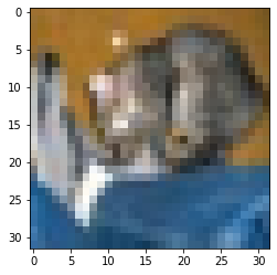
To verify that the dataset looks correct, let's plot the first images from the test set and display the image.

plt.imshow(X_test[0])

<matplotlib.image.AxesImage at 0x7fc1e4167ed0>

y_test

array([[3],
       [8],
       [8],
       ...,
       [5],
       [1],
       [7]], dtype=uint8)

Build CNN Model

The 8 lines of code below define the convolutional base using a common pattern: a stack of Conv2D ,MaxPooling2D , Dropout,Flatten and Dense layers.

As input, a Conv2D takes tensors of shape (image_height, image_width, color_channels), ignoring the batch size.In this example, you will configure our conv2D to process inputs of shape (32, 32, 3), which is the format of CIFAR images.

Maxpool2D() layer Downsamples the input representation by taking the maximum value over the window defined by pool_size(2,2) for each dimension along the features axis. The window is shifted by strides(2) in each dimension. The resulting output when using "valid" padding option has a shape.

Dropout() is used to by randomly set the outgoing edges of hidden units to 0 at each update of the training phase. The value passed in dropout specifies the probability at which outputs of the layer are dropped out.

Flatten() is used to convert the data into a 1-dimensional array for inputting it to the next layer.

Dense() layer is the regular deeply connected neural network layer with 128 neurons. The output layer is also a dense layer with 10 neurons for the 10 classes.

The activation function used is softmax. Softmax converts a real vector to a vector of categorical probabilities. The elements of the output vector are in range (0, 1) and sum to 1. Softmax is often used as the activation for the last layer of a classification network because the result could be interpreted as a probability distribution.

model = Sequential()
model.add(Conv2D(filters=32, kernel_size=(3, 3), padding='same', activation='relu', input_shape = [32, 32, 3]))

model.add(Conv2D(filters=32, kernel_size=(3, 3), padding='same', activation='relu'))
model.add(MaxPool2D(pool_size=(2,2), strides=2, padding='valid'))
model.add(Dropout(0.5))




model.add(Flatten())
model.add(Dense(units = 128, activation='relu'))
model.add(Dense(units=10, activation='softmax'))

model.summary()

Model: "sequential"
_________________________________________________________________
Layer (type)                 Output Shape              Param #   
=================================================================
conv2d (Conv2D)              (None, 32, 32, 32)        896       
_________________________________________________________________
conv2d_1 (Conv2D)            (None, 32, 32, 32)        9248      
_________________________________________________________________
max_pooling2d (MaxPooling2D) (None, 16, 16, 32)        0         
_________________________________________________________________
dropout (Dropout)            (None, 16, 16, 32)        0         
_________________________________________________________________
flatten (Flatten)            (None, 8192)              0         
_________________________________________________________________
dense (Dense)                (None, 128)               1048704   
_________________________________________________________________
dense_1 (Dense)              (None, 10)                1290      
=================================================================
Total params: 1,060,138
Trainable params: 1,060,138
Non-trainable params: 0
_________________________________________________________________

Compile and train the model

Here we are compiling the model and fitting it to the training data. We will use 10 epochs to train the model. An epoch is an iteration over the entire data provided. validation_data is the data on which to evaluate the loss and any model metrics at the end of each epoch. The model will not be trained on this data. As metrics = ['sparse_categorical_accuracy'] the model will be evaluated based on the accuracy.

model.compile(optimizer='adam', loss = 'sparse_categorical_crossentropy', metrics=['sparse_categorical_accuracy'])

history = model.fit(X_train, y_train, batch_size=10, epochs=10, verbose=1, validation_data=(X_test, y_test))

Train on 50000 samples, validate on 10000 samples
Epoch 1/10
50000/50000 [==============================] - 177s 4ms/sample - loss: 1.4127 - sparse_categorical_accuracy: 0.4918 - val_loss: 1.1079 - val_sparse_categorical_accuracy: 0.6095
Epoch 2/10
50000/50000 [==============================] - 159s 3ms/sample - loss: 1.1058 - sparse_categorical_accuracy: 0.6091 - val_loss: 1.0284 - val_sparse_categorical_accuracy: 0.6377
Epoch 3/10
50000/50000 [==============================] - 146s 3ms/sample - loss: 0.9946 - sparse_categorical_accuracy: 0.6477 - val_loss: 0.9682 - val_sparse_categorical_accuracy: 0.6564

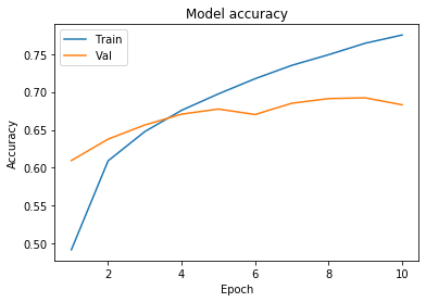
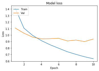
We will now plot the model accuracy and model loss. In model accuracy we will plot the training accuracy and validation accuracy and in model loss we will plot the training loss and validation loss.

# Plot training & validation accuracy values
epoch_range = range(1, 11)
plt.plot(epoch_range, history.history['sparse_categorical_accuracy'])
plt.plot(epoch_range, history.history['val_sparse_categorical_accuracy'])
plt.title('Model accuracy')
plt.ylabel('Accuracy')
plt.xlabel('Epoch')
plt.legend(['Train', 'Val'], loc='upper left')
plt.show()

# Plot training & validation loss values
plt.plot(epoch_range, history.history['loss'])
plt.plot(epoch_range, history.history['val_loss'])
plt.title('Model loss')
plt.ylabel('Loss')
plt.xlabel('Epoch')
plt.legend(['Train', 'Val'], loc='upper left')
plt.show()

test_loss, test_acc = model.evaluate(X_test,  y_test, verbose=2)

10000/10000 - 5s - loss: 0.9383 - sparse_categorical_accuracy: 0.6830

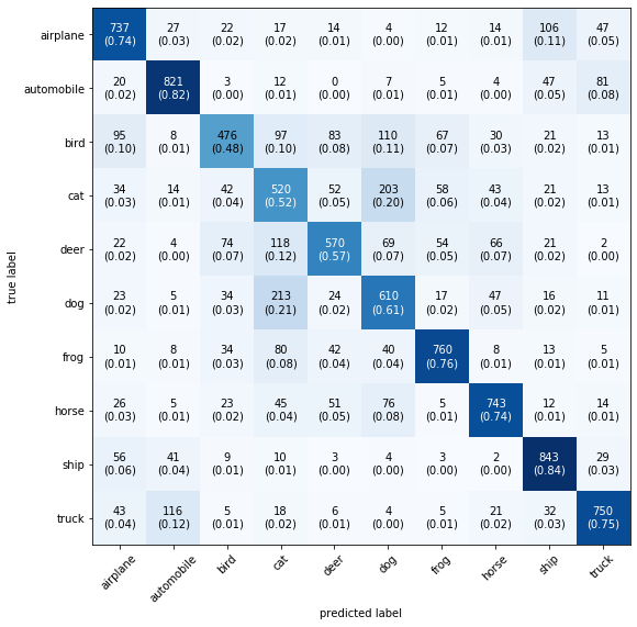
from mlxtend.plotting import plot_confusion_matrix
from sklearn.metrics import confusion_matrix

y_pred = model.predict_classes(X_test)

y_pred

array([3, 8, 8, ..., 5, 1, 7])

y_test

array([[3],
       [8],
       [8],
       ...,
       [5],
       [1],
       [7]], dtype=uint8)

mat = confusion_matrix(y_test, y_pred)
mat

array([[737,  27,  22,  17,  14,   4,  12,  14, 106,  47],
       [ 20, 821,   3,  12,   0,   7,   5,   4,  47,  81],
       [ 95,   8, 476,  97,  83, 110,  67,  30,  21,  13],
       [ 34,  14,  42, 520,  52, 203,  58,  43,  21,  13],
       [ 22,   4,  74, 118, 570,  69,  54,  66,  21,   2],
       [ 23,   5,  34, 213,  24, 610,  17,  47,  16,  11],
       [ 10,   8,  34,  80,  42,  40, 760,   8,  13,   5],
       [ 26,   5,  23,  45,  51,  76,   5, 743,  12,  14],
       [ 56,  41,   9,  10,   3,   4,   3,   2, 843,  29],
       [ 43, 116,   5,  18,   6,   4,   5,  21,  32, 750]])

plot_confusion_matrix(mat,figsize=(9,9), class_names=classes_name, show_normed=True)

(<Figure size 648x648 with 1 Axes>,
 <matplotlib.axes._subplots.AxesSubplot at 0x7fc12758d910>)

Conclusion:

In this tutorial we are have trained the simple Convolutional Neural Network (CNN) to classify CIFAR images.From the plot of learning curve we have observed that after 3 epoch the validation accuracy is less than the training set accuracy that refers to that our model is overfitting , which means we have increased the complexity of model. Also evaluated the model using confusion matrix. Observed that the model has predicted lower accuracy for bird, cat, deer, dog etc.. labels.