Matplotlib is a comprehensive library for creating static, animated, and interactive visualizations in Python. It is a cross-platform library for making 2D plots from data in arrays. It can be used in Python and IPython shells, Jupyter notebook and web application servers also. Matplotlib is written in Python and makes use of NumPy, the numerical mathematics extension of Python.

Here we have imported the necessary libraries.

import matplotlib.pyplot as plt
import numpy as np
from numpy.random import randint
%matplotlib inline

Plot

linspace() returns evenly spaced numbers over a specified interval. We will generate 20 evenly spaced numbers between 1 and 10.

x = np.linspace(1, 10, 20)
x

array([ 1.        ,  1.47368421,  1.94736842,  2.42105263,  2.89473684,
        3.36842105,  3.84210526,  4.31578947,  4.78947368,  5.26315789,
        5.73684211,  6.21052632,  6.68421053,  7.15789474,  7.63157895,
        8.10526316,  8.57894737,  9.05263158,  9.52631579, 10.        ])

The randint() method returns an integer number selected from the specified range. Here we are generating 20 random integers between 1 and 50.

y = randint(1, 50, 20)
y

array([43, 13, 39, 35, 14, 31, 36, 17, 27, 36, 15, 47, 12, 36,  6, 20, 19,
       17, 29, 36])

We can check the size of y as shown below.

y.size

20

You can get a list of all the functions which can be used on plt by running the command dir(plt).

dir(plt)[:10]

['Annotation',
 'Arrow',
 'Artist',
 'AutoLocator',
 'Axes',
 'Button',
 'Circle',
 'Figure',
 'FigureCanvasBase',
 'FixedFormatter']

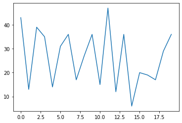
Now we will draw a plot for y using plt.plot().

plt.plot(y)

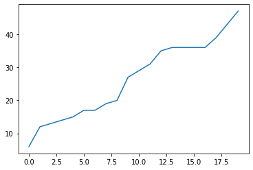
Now we will arrange the values in y ascending order using sort().

y = np.sort(y)
print(y)

[ 6 12 13 14 15 17 17 19 20 27 29 31 35 36 36 36 36 39 43 47]

plt.plot(y)

Label

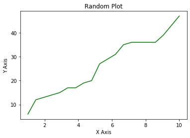
Till now we have only passed one parameter y to plot(). Hence the values on the x axis are not in our control. Now we will pass two parameter x and y to plot(). We have set the colour to green by passing color = 'g'. We can name the x and y axis by using xlabel() and ylabel(). We can even give a title to our plot using title().

plt.plot(x, y, color = 'g')
plt.xlabel('X Axis')
plt.ylabel('Y Axis')
plt.title('Random Plot')
plt.show()

Scatter, Bar, Hist, and Box Plots

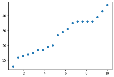
A scatter plot is a diagram where each value in the data set is represented by a dot. We can use scatter() to plot a scatter plot.

plt.scatter(x, y)

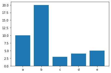
Now we will see how to plot a bar plot. For that first we will create the data a and b. Then we will draw the bar plot using bar().

b = [10, 20, 3, 4, 5]
a = ['a', 'b', 'c', 'd', 'e']
plt.bar(a, b)

sample() is an inbuilt function of random module in Python that returns a particular length list of items chosen from the sequence i.e. list, tuple, string or set. Here we are going to sample 10 integers from 1 to 10000.

from random import sample
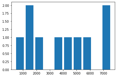
data = sample(range(1, 10000), 10)
data

[5768, 405, 2213, 7584, 5100, 1136, 7028, 1777, 3683, 4265]

Now we will draw a histogram for data using hist(). rwidth is used to set the relative width of the bars as a fraction of the bin width.

plt.hist(data, rwidth=0.8)

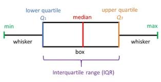
Now we will plot a box plot. Box plots show the five-number summary of a set of data: including the minimum, first (lower) quartile, median, third (upper) quartile, and maximum. Box plots divide the data into sections that each contain approximately 25% of the data in that set. The first quartile is the 25th percentile. Second quartile is 50th percentile and third quartile is 75th percentile.

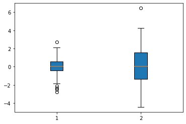
We will start by generating data. normal is used to draw random samples from a normal (Gaussian) distribution. It will draw 100 samples with mean 0 and standard deviation 1 and 2. We will use boxplot(). vert = True makes the boxes vertical. As patch_artist= True the boxes will be drawn using patch artists. A patch is a 2D artist with a face color and an edge color.

data = [np.random.normal(0, std, 100) for std in range(1,3)]
plt.boxplot(data, vert = True, patch_artist= True)
plt.show()

Subplot

Now we will see how to draw 2 plots together. For this we will use subplot(). It adds a subplot to the current figure. The first 2 parameters represent the number of rows and columns and the third parameter represents the index. Here we have one row and 2 columns. At the first index i.e at the first row and first column we are drawing x vs y plot. At the second index i.e. at the first row and second column we are drawing x vs x*y plot. We can use markersize to adjust the width of the point markers. b* represents blue stars.

plt.subplot(1, 2, 1)
plt.plot(x, y, 'ro', markersize = 5)

plt.subplot(1, 2, 2)
y2 = y*x
plt.plot(x, y2, 'b*')

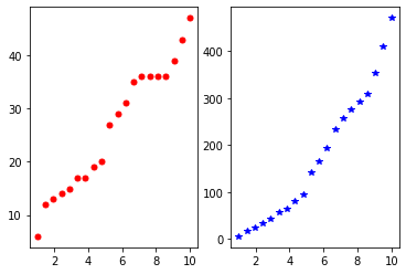
Now we will see the object oriented way to draw plots. We will first create a object and then call different methods on that object. Here we have created objects using plt.subplots() and then we are calling the method plot() on the object to get the line plot.

fig, ax = plt.subplots()
ax.plot(x, y, markersize = 12, linewidth = 3, color = '#005425')

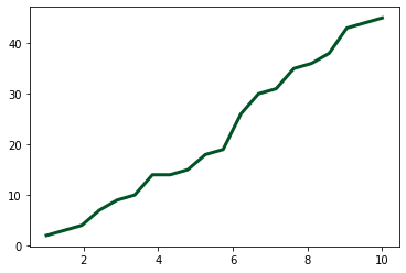
Now we will create a fig object using plt.figure(). Then we will add axes on the object using fig.add_axes() It add an axes at position rect [left, bottom, width, height]. Now we will draw two plots. We will plot x vs y on ax1 and x vs y2 i.e. x*y on ax2.

fig = plt.figure()
ax1 = fig.add_axes([0, 0, 1, 1])
ax2 = fig.add_axes([0.1, 0.6, 0.4, 0.3])


ax1.plot(x, y, 'r')
ax1.set_xlabel('X')
ax1.set_ylabel('Y')
ax1.set_title('Y Plot')

ax2.plot(x, y2, 'g')
ax2.set_xlabel('X')
ax2.set_ylabel('Y')
ax2.set_title('Y2 Plot')

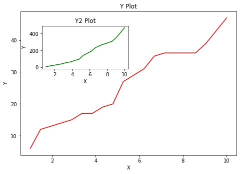
Here we have created objects fig and ax. We will create 2 subplots using subplots(1,2) i.e. we will have one row and 2 columns. ax[0] gives us the first position i.e. first row and first column. ax[1] gives us the second position i.e. first row and second column.

fig, ax = plt.subplots(1,2)

ax[0].plot(x, y, 'b')

ax[1].plot(x, y, 'r')

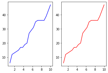
Now we will use a for loop which is more efficient way to do the same thing. In the first iteration of the loop x vs y plot is drawn using red colour in the first position. In the second loop x vs y2 plot is drawn using green colour in the second position. tight_layout() will adjust spacing between subplots to minimize the overlaps.

fig, ax = plt.subplots(1, 2)
col = ['r', 'g']
data = [y, y2]

for i, axes in enumerate(ax):
    axes.plot(x, data[i], col[i])

fig.tight_layout()

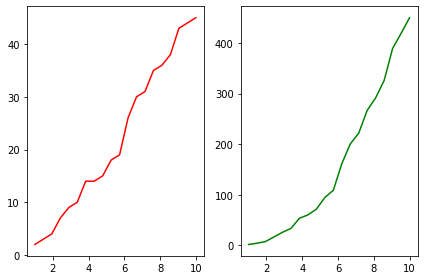
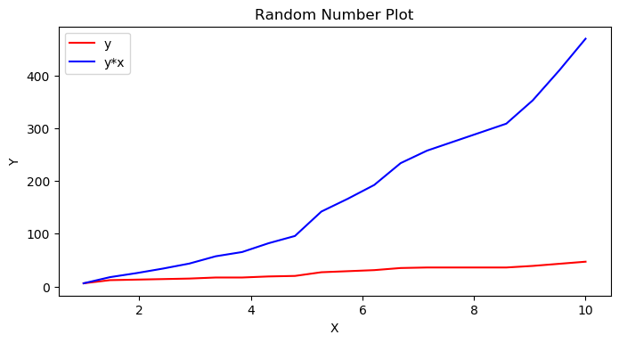
We can change the figure size using figsize. We can even control the resolution in dots per inch using dpi. Here we have plotted 2 lines having same x axis in the same plot. A legend is an area describing the elements of the graph. In the matplotlib library, there's a function called legend() which is used to Place a legend on the axes. The attribute loc in legend() is used to specify the location of the legend. Finally, we can save the current figure using savefig() method on the fig object

fig, ax = plt.subplots(figsize = (8,4), dpi = 100)

ax.plot(x, y, 'r', label = 'y')
ax.plot(x, y2, 'b', label = 'y*x')
ax.set_xlabel('X')
ax.set_ylabel('Y')
ax.set_title('Random Number Plot')
ax.legend(loc = 0)
fig.savefig('random file.png', dpi = 100)

xlim, ylim, xticks, and yticks

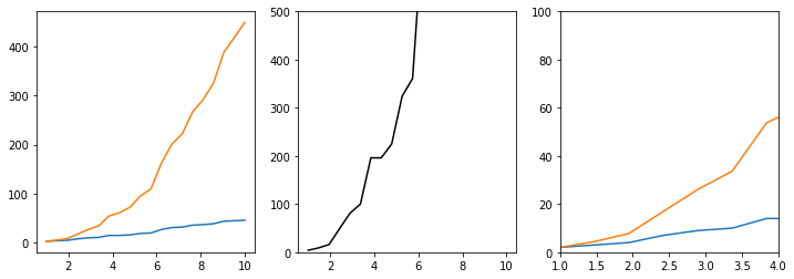
As you can see we have got 2 plots in a single axes by passing two pairs of x and y values. We are limiting the x and y axis values using set_xlim() and set_ylim() respectively. The first subplot and the third subplot have the same values but different x and y limits. We can say that the third subplot is the zoomed version of the first subplot.

fig, ax = plt.subplots(1, 3, figsize = (12, 4))

ax[0].plot(x, y, x, y2)

ax[1].plot(x, y**2, 'k')
ax[1].set_ylim([0, 500])

ax[2].plot(x, y, x, y2)
ax[2].set_ylim([0, 100])
ax[2].set_xlim([1 ,4])

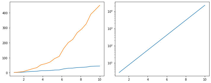
Now we will see how to change the scale type. We can change the scale of y axis by using set_yscale(). We have set the y scale type to log which is the logarithmic scale. The exp() function in Python allows users to calculate the exponential value with the base set to e.

fig, ax = plt.subplots(1, 2, figsize= (10, 4))
ax[0].plot(x, y, x, y2)

ax[1].plot(x, np.exp(x))
ax[1].set_yscale('log')
fig.tight_layout()

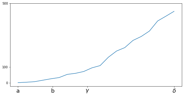
Now we will see how to format the ticks. Ticks are the values used to show specific points on the coordinate axis. set_xticks() is used to set the current tick locations on the x axis. set_xticklabels() is used to set the current tick labels of the x-axis.

fig, ax = plt.subplots(figsize = (10,5))
ax.plot(x, y2)
ax.set_xticks([1 , 3, 5, 10])
ax.set_xticklabels([r'a', r'b', r'$\gamma$', r'$\delta$'], fontsize=18)

ax.set_yticks([0, 100, 500])

Here we are importing the ticker module. This module contains classes for configuring tick locating and formatting.

from matplotlib import ticker

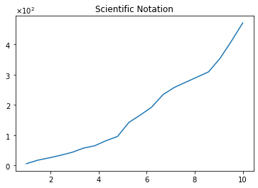
ScalarFormatter is a default formatter for scalars. It formats tick values as a number. As useMathText=True it will show the offset in a latex-like (MathText) format as x10^2. set_scientific() is used to turn scientific notation on or off. Here scientific notation is on. set_powerlimits() is used to set size thresholds for scientific notation.

fig, ax = plt.subplots()
ax.plot(x, y2)
ax.set_title('Scientific Notation')

formatter = ticker.ScalarFormatter(useMathText=True)
formatter.set_scientific(True)
formatter.set_powerlimits((-1, 2))
ax.yaxis.set_major_formatter(formatter)