Airline Passenger Prediction using RNN – LSTM
Prediction of number of passengers for an airline using LSTM
In this project we are going to build a model to predict the number of passengers in an airline. To do so we are going to use Recurrent Neural Networks, more precisely Long Short Term Memory.
Recurrent Neural Network
- Neural Networks are set of algorithms which closely resembles the human brain and are designed to recognize patterns.
- Recurrent Neural Network is a generalization of feedforward neural network that has an internal memory.
- RNN is recurrent in nature as it performs the same function for every input of data while the output of the current input depends on the past one computation.
- After producing the output, it is copied and sent back into the recurrent network. For making a decision, it considers the current input and the output that it has learned from the previous input.
- In other neural networks, all the inputs are independent of each other. But in RNN, all the inputs are related to each other.
Long Short Term Memory
- Long Short-Term Memory (LSTM) networks are a modified version of recurrent neural networks, which makes it easier to remember past data in memory.
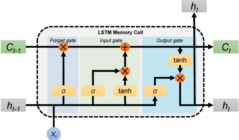
- Generally LSTM is composed of a cell (the memory part of the LSTM unit) and three “regulators”, usually called gates, of the flow of information inside the LSTM unit: an input gate, an output gate and a forget gate.
- Intuitively, the cell is responsible for keeping track of the dependencies between the elements in the input sequence.
- The input gate controls the extent to which a new value flows into the cell, the forget gate controls the extent to which a value remains in the cell and the output gate controls the extent to which the value in the cell is used to compute the output activation of the LSTM unit.
- The activation function of the LSTM gates is often the logistic sigmoid function.
- There are connections into and out of the LSTM gates, a few of which are recurrent. The weights of these connections, which need to be learned during training, determine how the gates operate.
Dataset
This dataset provides monthly totals of a US airline passengers from 1949 to 1960. The dataset has 2 columns month and passengers. month contains the month of the year and passengers contains total number of passengers travelled on that particular month.
You can download the dataset from here.
We are going to use tensorflow to build the LSTM. You can install tensorflow by running this command. If you machine has a GPU you can use the second command.
!pip install tensorflow
!pip install tensorflow-gpu
The necessary python libraries are imported here-
numpyis used to perform basic array operationspyplotfrom matplotlib is used to visualize the resultspandasfor loading and manipulating the data.Tensorflowis used to build the neural network- We have even imported all the layers required to build the model from
keras.
import numpy as np
import matplotlib.pyplot as plt
import pandas as pd
from tensorflow.keras.models import Sequential
from tensorflow.keras.layers import Dense, LSTM
from sklearn.preprocessing import MinMaxScaler
Now we will read the dataset using read.csv(). We will only retain the passengers column from the dataset and reshape it by converting it into a numpy array.
dataset = pd.read_csv('AirPassengers.csv')
dataset = dataset['#Passengers']
dataset = np.array(dataset).reshape(-1,1)
dataset[:10]
array([[112],
[118],
[132],
[129],
[121],
[135],
[148],
[148],
[136],
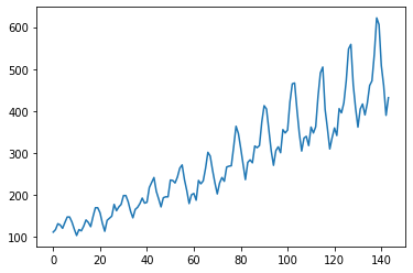
[119]], dtype=int64)Now we will plot the dataset. We can observe that the number of passengers has increased linearly.
plt.plot(dataset)
Neural networks work better if inputs are between 0 and 1. So we are going to scale down the inputs using MinMaxScaler(). We can see that after scaling the minimum value is 0 and maximum value is 1.
scaler = MinMaxScaler()
dataset = scaler.fit_transform(dataset)
dataset.min(),dataset.max()
(0.0, 1.0)
We are going to use the data of first 100 months as training data and the last 44 months as testing data.
train_size = 100
test_size = 44
train = dataset[0:train_size, :]
train.shape
(100, 1)
test = dataset[train_size:144, :]
test.shape
(44, 1)
Create training and testing dataset
We are going to predict the (i)th value in the dataset on the basis of (i-1)th value. That means we are going to look back by 1 to predict the next value. Hence we are creating a function get_data() to create dataX and dataY for the training as well as the testing data.
def get_data(dataset, look_back):
    dataX, dataY = [], []
    for i in range(len(dataset)-look_back-1):
        a = dataset[i:(i+look_back), 0]
        dataX.append(a)
        dataY.append(dataset[i+look_back, 0])
    return np.array(dataX), np.array(dataY)

look_back = 1
X_train, y_train = get_data(train, look_back)
X_train[:10]
array([[0.01544402],
       [0.02702703],
       [0.05405405],
       [0.04826255],
       [0.03281853],
       [0.05984556],
       [0.08494208],
       [0.08494208],
       [0.06177606],
       [0.02895753]])
y_train[:10]
array([0.02702703, 0.05405405, 0.04826255, 0.03281853, 0.05984556,
       0.08494208, 0.08494208, 0.06177606, 0.02895753, 0.        ])
Now we have called get_data() to create the testing data.
X_test, y_test = get_data(test, look_back)
Now we are going to reshape our data and make it 2 dimensional using reshape().
X_train = X_train.reshape(X_train.shape[0], X_train.shape[1], 1)
X_test = X_test.reshape(X_test.shape[0], X_test.shape[1], 1)
X_train.shape
(98, 1, 1)
Build the model
Our sequential model has 2 layers
LSTM layer:
This is the main layer of the model and has 5 units. It learns long-term dependencies between time steps in time series and sequence data. input_shape contains the shape of input which we have to pass as a parameter to the first layer of our neural network.
Dense layer:
Dense layer is the regular deeply connected neural network layer. It is most common and frequently used layer. We have number of units as 1 because we are going to get a single value as the output.
model = Sequential()
model.add(LSTM(5, input_shape = (1, look_back)))
model.add(Dense(1))
model.compile(loss = 'mean_squared_error', optimizer = 'adam')
We have compliled the model. We can see the summary using model.summary().
model.summary()
Model: "sequential"
_________________________________________________________________
Layer (type)                 Output Shape              Param #
=================================================================
lstm (LSTM)                  (None, 5)                 140
_________________________________________________________________
dense (Dense)                (None, 1)                 6
=================================================================
Total params: 146
Trainable params: 146
Non-trainable params: 0
_________________________________________________________________
After compiling the model we will now train the model using model.fit() on the training dataset. We will use 50 epochs to train the model. An epoch is an iteration over the entire x and y data provided. batch_size is the number of samples per gradient update i.e. the weights will be updates after every training example.
model.fit(X_train, y_train, epochs=50, batch_size=1)

Epoch 45/50
98/98 [==============================] - 0s 2ms/sample - loss: 0.0022
Epoch 46/50
98/98 [==============================] - 0s 2ms/sample - loss: 0.0021
Epoch 47/50
98/98 [==============================] - 0s 2ms/sample - loss: 0.0021
Epoch 48/50
98/98 [==============================] - 0s 2ms/sample - loss: 0.0021
Epoch 49/50
98/98 [==============================] - 0s 2ms/sample - loss: 0.0022
Epoch 50/50
98/98 [==============================] - 0s 2ms/sample - loss: 0.0021
Now we will test our model using X_test.
y_pred = model.predict(X_test)
This is the scaler value which we had used earlier.
scaler.scale_
array([0.0019305])
We had scaled down the values in our dataset before passing it to the neural network. Now we will have to get the original values back. For this we will use scaler.inverse_transform().
y_pred = scaler.inverse_transform(y_pred)
y_test = np.array(y_test)
y_test = y_test.reshape(-1, 1)
y_test = scaler.inverse_transform(y_test)
Now we will visualize the result by plotting the real values and the predicted values.
# plot baseline and predictions
plt.figure(figsize=(14,5))
plt.plot(y_test, label = 'Real number of passengers')
plt.plot(y_pred, label = 'Predicted number of passengers')
plt.ylabel('# passengers')
plt.legend()
plt.show()
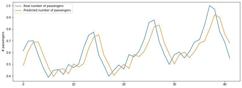
As we can see that the actual results and the predicted results are following the same trend. Our model is predicting the number of passengers with a good accuracy.
0 Comments