Deep Learning with TensorFlow 2.0 Tutorial – Building Your First ANN with TensorFlow 2.0
Deep learning with Tensorflow
# pip install tensorflow==2.0.0-rc0
# pip install tensorflow-gpu==2.0.0-rc0
Watch Full Lesson Here:
Objective
- Our objective for this code is to build to an Artificial neural network for classification problem using
tensorflowandkeraslibraries. We will try to learn how to build anerual netwroks model usingtensorflowandkerasthen we will analyse our model using differentaccuracy metrics.
What is ANN?
Artificial Neural Networks (ANN) is a supervised learning system built of a large number of simple elements, called neurons or perceptrons. Each neuron can make simple decisions, and feeds those decisions to other neurons, organized in interconnected layers.


What is Activation Function?
- In artificial neural networks, the
activation functionof a node defines the output of that node given an input or set of inputs. A standard integrated circuit can be seen as a digital network of activation functions that can be “ON” (1) or “OFF” (0), depending on input. This is similar to the behavior of the linear perceptron in neural networks. - If we do not apply a Activation function then the output signal would simply be a simple linear function.A linear function is just a polynomial of one degree.
Types of Activation Function
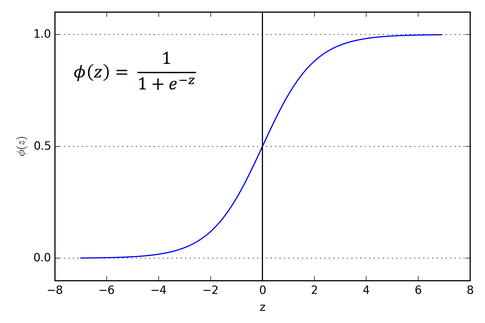
- Sigmoid
- Tanh
- ReLu
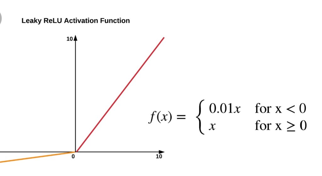
- LeakyReLu
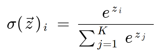
- SoftMax
Sigmoid


Softmax Funcation
What is Back Propagation?
- In
backpropagationwe update the parameters of the model with respect toloss function. Loss function can becross entropyforclassificationproblem androot mean squared errorforregressionproblems. - Our objective is to
minimize lossof our model. So to minimize loss of our model we caluculategradeint of losswith respect toparamtersof model and try to minimize the this gradient. while minimizing the gradient we update the weights of our model this process is known as back propagation.

Steps for building your first ANN
- Data Preprocessing
- Add input layer
- Random w init
- Add Hidden Layers
- Select Optimizer, Loss, and Performance Metrics
- Compile the model
- use model.fit to train the model
- Evaluate the model
- Adjust optimization parameters or model if needed
Data Preprocessing
- It is better to preprocess data before giving it to any neural net model. Data should be
normally distributed(gaussian distribution), so that model performs well. - If our data is not normally distributed that means there is
skewnessin data. To remove skewness of data we can take logarithm of data . by using log function we can remove skewness of data. - After removing skewness of data it is better to scale of data so that all values are at same scale.
- We can either use
MinMax scalerorStandardscaler. - Standardscalers are better to use since by using it mean and variance of our data is now 0 and 1 respectively . That is now our data is in form of N(0,1) that is gaussian distribution with mean 0 and variance 1.
Layers
Adding input layer
- according to size of our input we add number of input layers.
Adding hidden layers
- We can add as many hidden layers. if we want our model to be complex than large number of hidden layers can be added and for simple model number of hidden layes can be small
Adding output layer
- In a
classification problemsize of output layer depend on number of classes. - In
regression problemthere is size of output layer is one
Weight initialization
- The
meanof the weights should be zero. - The
varianceof the weights should stay the same across every layer.
Optimizers
Gradient Descent
- Gradient descent is a first-order optimization algorithm which is dependent on the first order derivative of a loss function. It calculates that which way the weights should be altered so that the function can reach a minima. Through backpropagation, the loss is transferred from one layer to another and the model’s parameters also known as weights are modified depending on the losses so that the loss can be minimized.
Stochastic Gradient Descent
- It’s a variant of Gradient Descent. It tries to update the model’s parameters more frequently. In this, the model parameters are altered after computation of loss on each training example. So, if the dataset contains 1000 rows SGD will update the model parameters 1000 times in one cycle of dataset instead of one time as in Gradient Descent.
Mini-Batch Gradient Descent
- It’s best among all the variations of gradient descent algorithms. It is an improvement on both SGD and standard gradient descent. It updates the model parameters after every batch. So, the dataset is divided into various batches and after every batch, the parameters are updated.
Adagrad
- It is gradient descent with adaptive learning rate
- in this the learning rate decays for parameters in proportion to their update history(more updates means more decay)
losses
Cross entropyfor Classification problems.Root mean squarederror for regression problems.
Accuracy metrics
\begin{align*}
Accuracy  = \frac{TP + TN }{TP+FP+TN+FN}
\end{align*}
\begin{align*}
Recall  = \frac{TP}{TP+FN}
\end{align*}
\begin{align*}
Precision  = \frac{TP}{TP+FP}
\end{align*}
Installing libraries
# pip install tensorflow==2.0.0-rc0
# pip install tensorflow-gpu==2.0.0-rc0
import tensorflow as tf
from tensorflow import keras
from tensorflow.keras import Sequential
from tensorflow.keras.layers import Flatten, Dense
print(tf.__version__)
2.2.0
Importing necessary libraries
import numpy as np
import pandas as pd
from sklearn.model_selection import train_test_split
dataset = pd.read_csv('Customer_Churn_Modelling.csv')
dataset.head()
| RowNumber | CustomerId | Surname | CreditScore | Geography | Gender | Age | Tenure | Balance | NumOfProducts | HasCrCard | IsActiveMember | EstimatedSalary | Exited | |
|---|---|---|---|---|---|---|---|---|---|---|---|---|---|---|
| 0 | 1 | 15634602 | Hargrave | 619 | France | Female | 42 | 2 | 0.00 | 1 | 1 | 1 | 101348.88 | 1 |
| 1 | 2 | 15647311 | Hill | 608 | Spain | Female | 41 | 1 | 83807.86 | 1 | 0 | 1 | 112542.58 | 0 |
| 2 | 3 | 15619304 | Onio | 502 | France | Female | 42 | 8 | 159660.80 | 3 | 1 | 0 | 113931.57 | 1 |
| 3 | 4 | 15701354 | Boni | 699 | France | Female | 39 | 1 | 0.00 | 2 | 0 | 0 | 93826.63 | 0 |
| 4 | 5 | 15737888 | Mitchell | 850 | Spain | Female | 43 | 2 | 125510.82 | 1 | 1 | 1 | 79084.10 | 0 |
X = dataset.drop(labels=['CustomerId', 'Surname', 'RowNumber', 'Exited'], axis = 1)
y = dataset['Exited']
X.head()
| CreditScore | Geography | Gender | Age | Tenure | Balance | NumOfProducts | HasCrCard | IsActiveMember | EstimatedSalary | |
|---|---|---|---|---|---|---|---|---|---|---|
| 0 | 619 | France | Female | 42 | 2 | 0.00 | 1 | 1 | 1 | 101348.88 |
| 1 | 608 | Spain | Female | 41 | 1 | 83807.86 | 1 | 0 | 1 | 112542.58 |
| 2 | 502 | France | Female | 42 | 8 | 159660.80 | 3 | 1 | 0 | 113931.57 |
| 3 | 699 | France | Female | 39 | 1 | 0.00 | 2 | 0 | 0 | 93826.63 |
| 4 | 850 | Spain | Female | 43 | 2 | 125510.82 | 1 | 1 | 1 | 79084.10 |
y.head()
0    1
1    0
2    1
3    0
4    0
Name: Exited, dtype: int64
Using label encoder we are converting categorical features to numerical features
from sklearn.preprocessing import LabelEncoder
label1 = LabelEncoder()
X['Geography'] = label1.fit_transform(X['Geography'])
label = LabelEncoder()
X['Gender'] = label.fit_transform(X['Gender'])
X.head()
| CreditScore | Geography | Gender | Age | Tenure | Balance | NumOfProducts | HasCrCard | IsActiveMember | EstimatedSalary | |
|---|---|---|---|---|---|---|---|---|---|---|
| 0 | 619 | 0 | 0 | 42 | 2 | 0.00 | 1 | 1 | 1 | 101348.88 |
| 1 | 608 | 2 | 0 | 41 | 1 | 83807.86 | 1 | 0 | 1 | 112542.58 |
| 2 | 502 | 0 | 0 | 42 | 8 | 159660.80 | 3 | 1 | 0 | 113931.57 |
| 3 | 699 | 0 | 0 | 39 | 1 | 0.00 | 2 | 0 | 0 | 93826.63 |
| 4 | 850 | 2 | 0 | 43 | 2 | 125510.82 | 1 | 1 | 1 | 79084.10 |
X = pd.get_dummies(X, drop_first=True, columns=['Geography'])
X.head()
| CreditScore | Gender | Age | Tenure | Balance | NumOfProducts | HasCrCard | IsActiveMember | EstimatedSalary | Geography_1 | Geography_2 | |
|---|---|---|---|---|---|---|---|---|---|---|---|
| 0 | 619 | 0 | 42 | 2 | 0.00 | 1 | 1 | 1 | 101348.88 | 0 | 0 |
| 1 | 608 | 0 | 41 | 1 | 83807.86 | 1 | 0 | 1 | 112542.58 | 0 | 1 |
| 2 | 502 | 0 | 42 | 8 | 159660.80 | 3 | 1 | 0 | 113931.57 | 0 | 0 |
| 3 | 699 | 0 | 39 | 1 | 0.00 | 2 | 0 | 0 | 93826.63 | 0 | 0 |
| 4 | 850 | 0 | 43 | 2 | 125510.82 | 1 | 1 | 1 | 79084.10 | 0 | 1 |
- Here using standardscaler we are scaling our data, we are scaling such that the mean is 0 and variance is 1 for data
from sklearn.preprocessing import StandardScaler
X_train, X_test, y_train, y_test = train_test_split(X, y, test_size = 0.2, random_state = 0, stratify = y)
scaler = StandardScaler()
X_train = scaler.fit_transform(X_train)
X_test = scaler.transform(X_test)
X_train
array([[-1.24021723, -1.09665089,  0.77986083, ...,  1.64099027,
        -0.57812007, -0.57504086],
       [ 0.75974873,  0.91186722, -0.27382717, ..., -1.55587522,
         1.72974448, -0.57504086],
       [-1.72725557, -1.09665089, -0.9443559 , ...,  1.1038111 ,
        -0.57812007, -0.57504086],
       ...,
       [-0.51484098,  0.91186722,  0.87565065, ..., -1.01507508,
         1.72974448, -0.57504086],
       [ 0.73902369, -1.09665089, -0.36961699, ..., -1.47887193,
        -0.57812007, -0.57504086],
       [ 0.95663657,  0.91186722, -1.32751517, ...,  0.50945854,
        -0.57812007,  1.73900686]])
Build ANN
- Here bwe are building ANN model.
- First we add input layer of shape of input that is 11 in this case.
- There is only one hidden layers whose shape is 128.
- Shape of Output layer is only 1 since we have only one output.
model = Sequential()
model.add(Dense(X.shape[1], activation='relu', input_dim = X.shape[1]))
model.add(Dense(128, activation='relu'))
model.add(Dense(1, activation = 'sigmoid'))
X.shape[1]
11
- Here we are compiling our model. we have selected Adam optimizer. loss is binary crossentropy and metric is accuracy
model.compile(optimizer='adam', loss = 'binary_crossentropy', metrics=['accuracy'])
- Here we are fitting model on training dataset . we have given bacth size of 10 and eopchs are 10
model.fit(X_train, y_train.to_numpy(), batch_size = 10, epochs = 10, verbose = 1)
Epoch 1/10
800/800 [==============================] - 1s 2ms/step - loss: 0.4516 - accuracy: 0.8116
Epoch 2/10
800/800 [==============================] - 1s 1ms/step - loss: 0.3948 - accuracy: 0.8372
Epoch 3/10
800/800 [==============================] - 1s 1ms/step - loss: 0.3597 - accuracy: 0.8543
Epoch 4/10
800/800 [==============================] - 1s 2ms/step - loss: 0.3475 - accuracy: 0.8576
Epoch 5/10
800/800 [==============================] - 1s 1ms/step - loss: 0.3426 - accuracy: 0.8611
Epoch 6/10
800/800 [==============================] - 1s 1ms/step - loss: 0.3389 - accuracy: 0.8619
Epoch 7/10
800/800 [==============================] - 1s 1ms/step - loss: 0.3366 - accuracy: 0.8625
Epoch 8/10
800/800 [==============================] - 1s 1ms/step - loss: 0.3350 - accuracy: 0.8629
Epoch 9/10
800/800 [==============================] - 1s 2ms/step - loss: 0.3333 - accuracy: 0.8635
Epoch 10/10
800/800 [==============================] - 1s 1ms/step - loss: 0.3311 - accuracy: 0.8634
<tensorflow.python.keras.callbacks.History at 0x271d1a03580>
- Using model.predict we predict output values for our input data.
y_pred = model.predict_classes(X_test)
y_pred
array([[0],
       [0],
       [0],
       ...,
       [0],
       [1],
       [0]])
y_test
1344    1
8167    0
4747    0
5004    1
3124    1
       ..
9107    0
8249    0
8337    0
6279    1
412     0
Name: Exited, Length: 2000, dtype: int64
model.evaluate(X_test, y_test.to_numpy())
63/63 [==============================] - 0s 2ms/step - loss: 0.3489 - accuracy: 0.8520
[0.34891313314437866, 0.8519999980926514]
from sklearn.metrics import confusion_matrix, accuracy_score
Confusion matrix
confusion_matrix(y_test, y_pred)
array([[1546,   47],
       [ 249,  158]], dtype=int64)
accuracy_score(y_test, y_pred)
0.852
Summary
- In this notebook we have implemented a classifer using artificial neural network. We build the model using tensorflow and keras. We checked the accuracy using Accuracy metrics and Confusion metrix. Accuracy for the model was 85.2% on test data.
3 Comments