What is Ensemble Learning?

We can define Ensemble Learning in this way it uses multiple machine learning models or multiple set of models for the same algorithm which try to make a better prediction.

Ensemble Learning model works by training different models on the same dataset and makes prediction iindividually and once the prediction is made then these results are combines with some statistical methods to get final prediction

In one sentence we can explain like this there is a dataset where multiple algorithms are trained on the same dataset and then finally predictions are made based on the outcomes of the individual machine learning algorithms.

Let me explain this with an example of cricket team, in cricket team or any other team every few players are specialized in some fields(batting, fast bowling, fielding, keeping, ... etc). In the same way every algorithm has its own feature set. There are multiple algorithms and they are specialized in some way so once we combine all of these algorithms it's easy to get the final predictions.

Why Ensemble Learning

Now we will try to understand why we use Ensemble learning:

If we try to start with a simple model to achive high accuracy by using single algorithm it might be endup with overfitting or underfitting.

Every model has its own strength and weakness. If we combine multiple models it will help us to hide weakness of individual models sothat we can cover weakness of others.

It creates some errors, The error emerging from any machine model can be broken down into three components mathematically. Following are these component:

• Bias
• Variance
• Irreducible error

To understand these errors have a look at the following figure:

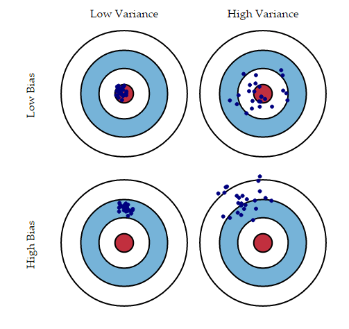
Bias error is useful to quantify how much on an average are the predicted values different from the actual value.

Variance on the other side quantifies how are the prediction made on the same observation different from each other.

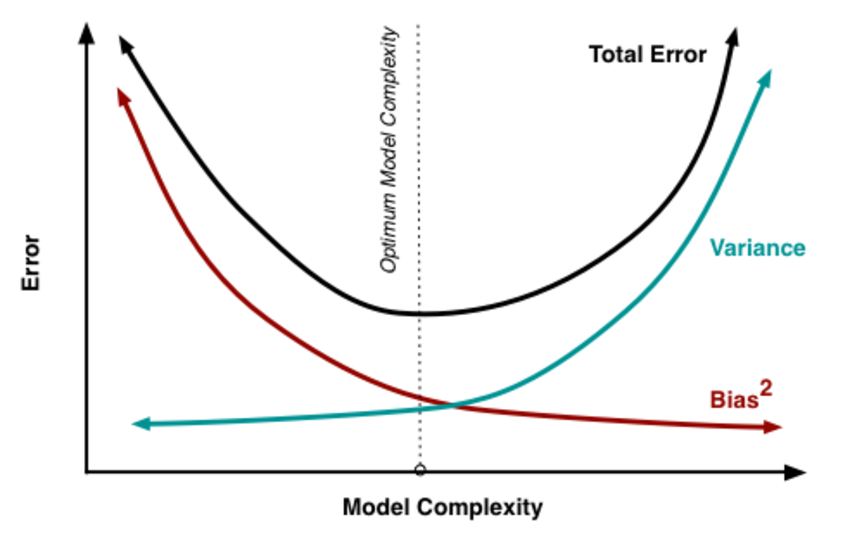
Now we will try to understand bias - variance trade off from the following figure.
By increasing model complexity, total error will decrease till some point and then it will start to increase. W need to select optimum model complexity to get less error.

For low complexity model : high bias and low variance
For high complexity model : low bias and high variance

If you are getting high bias then you have a fair chance to increase model complexity. And otherside it you are getting high variance, you need to decrease model complexity that's how any machine learning algorithm works.

Let's look into the types of Ensemble Learning:

Type of Ensemble Learning

• Basic Ensemble Techniques
  • Max Voting
  • Averaging
  • Weighted Average
• Advanced Ensemble Techniques
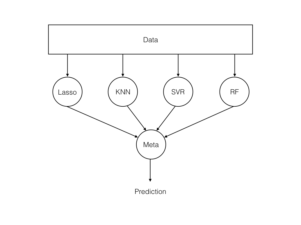
  • Stacking
  • Blending
  • Bagging
  • Boosting

• Algorithms based on Bagging
  • Bagging meta-estimator
  • Random Forest
• Boosting Algorithms
  • AdaBoost
  • GBM
  • XGB
  • Light GBM
  • CatBoost

Max Voting

The max voting method is generally used for classification problems. In this technique, multiple models are used to make predictions for each data point.

Averaging

Similar to the max voting technique, multiple predictions are made for each data point in averaging.

Weighted Average

This is an extension of the averaging method. All models are assigned different weights defining the importance of each model for prediction.

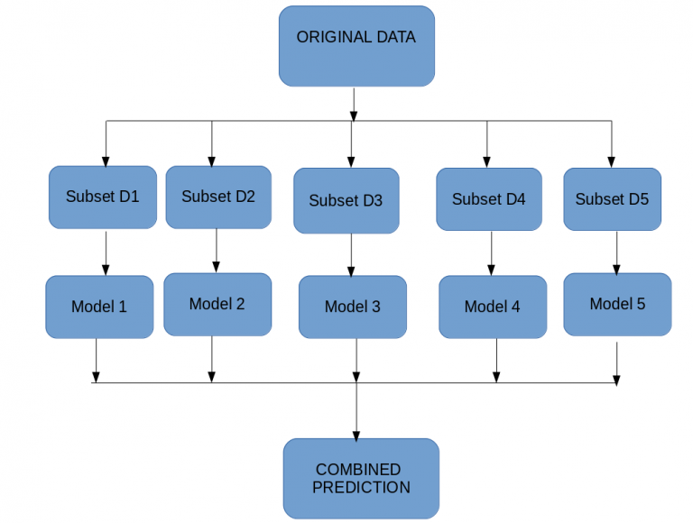
Bagging

Bagging is also known as Bootstrapping. It is a sampling technique in which we create subsets of observations from the original dataset, with replacement. The size of the subsets is the same as the size of the original set.

• combining predictions that belong to the same type.
• Aim to decrease variance, not bias.
• Different training data subsets are randomly drawn with replacement from the entire training dataset.

To explain bagging Random Forest(below figure) is the best example.
It creates multiple subsets like decision tree and it makes a prediction for each decision tree then if random forest is classifier it will take max voting otherwise if it is a regressor it will take avearge from each of these subset of the trees .

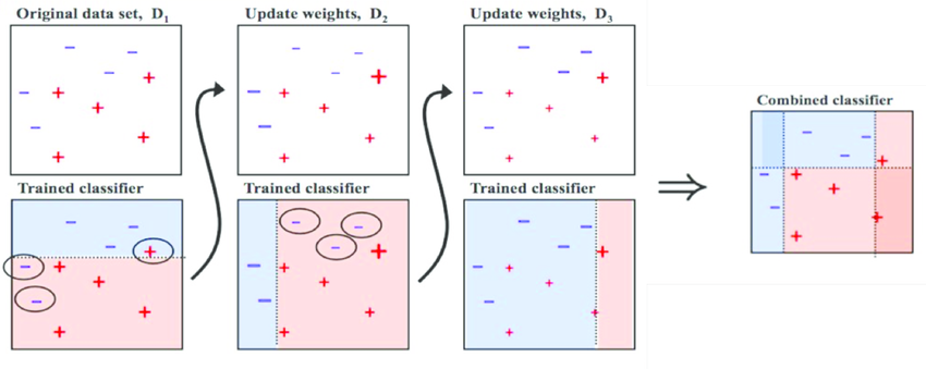
Boosting

Boosting is a sequential process, where each subsequent model attempts to correct the errors of the previous model. The succeeding models are dependent on the previous model.
Let’s understand the way boosting works in the below steps.

• Combining predictions that belong to the different types.
• Aim to decrease bias, not variance.
• Models are weighted according to their performance.

Let's now understand boosting from the following figure: At first we have our original dataset ,our first algorithm creates a plane there for that we have SVM classifier, Random Forest classifier, etc and it found out that there are some errors in the plane . To rectife that errors , we will train other model and after this again we will train other model which identifies errors.
Finally, we combine all three models together which perfectly classify our original dataset.

Algorithms Implimentation in sklearn

• Bagging
  • Random Forest
• Boosting
  • XGBosst
  • AdaBoost
  • Gradient Boosting

Random Forest is another ensemble machine learning algorithm that follows the bagging technique

XGBoost (extreme Gradient Boosting) is an advanced implementation of the gradient boosting algorithm

Adaptive boosting or AdaBoost is one of the simplest boosting algorithms

Gradient Boosting or GBM is another ensemble machine learning algorithm that works for both regression and classification problems

Data Preparation

Importing required libraries

import pandas as pd
import seaborn as sns
import matplotlib.pyplot as plt
import numpy as np

Loading the training data set

from sklearn import datasets, metrics
from sklearn.model_selection import train_test_split
from sklearn.preprocessing import StandardScaler

cancer = datasets.load_breast_cancer()

Let's go ahead and get the description the breast cancer data set.

print(cancer.DESCR)

.. _breast_cancer_dataset:

Breast cancer wisconsin (diagnostic) dataset
--------------------------------------------

**Data Set Characteristics:**

    :Number of Instances: 569

    :Number of Attributes: 30 numeric, predictive attributes and the class

    :Attribute Information:
        - radius (mean of distances from center to points on the perimeter)
        - texture (standard deviation of gray-scale values)
        - perimeter
        - area
        - smoothness (local variation in radius lengths)
        - compactness (perimeter^2 / area - 1.0)
        - concavity (severity of concave portions of the contour)
        - concave points (number of concave portions of the contour)
        - symmetry
        - fractal dimension ("coastline approximation" - 1)

        The mean, standard error, and "worst" or largest (mean of the three
        worst/largest values) of these features were computed for each image,
        resulting in 30 features.  For instance, field 0 is Mean Radius, field
        10 is Radius SE, field 20 is Worst Radius.

        - class:
                - WDBC-Malignant
                - WDBC-Benign

    :Summary Statistics:

    ===================================== ====== ======
                                           Min    Max
    ===================================== ====== ======
    radius (mean):                        6.981  28.11
    texture (mean):                       9.71   39.28
    perimeter (mean):                     43.79  188.5
    area (mean):                          143.5  2501.0
    smoothness (mean):                    0.053  0.163
    compactness (mean):                   0.019  0.345
    concavity (mean):                     0.0    0.427
    concave points (mean):                0.0    0.201
    symmetry (mean):                      0.106  0.304
    fractal dimension (mean):             0.05   0.097
    radius (standard error):              0.112  2.873
    texture (standard error):             0.36   4.885
    perimeter (standard error):           0.757  21.98
    area (standard error):                6.802  542.2
    smoothness (standard error):          0.002  0.031
    compactness (standard error):         0.002  0.135
    concavity (standard error):           0.0    0.396
    concave points (standard error):      0.0    0.053
    symmetry (standard error):            0.008  0.079
    fractal dimension (standard error):   0.001  0.03
    radius (worst):                       7.93   36.04
    texture (worst):                      12.02  49.54
    perimeter (worst):                    50.41  251.2
    area (worst):                         185.2  4254.0
    smoothness (worst):                   0.071  0.223
    compactness (worst):                  0.027  1.058
    concavity (worst):                    0.0    1.252
    concave points (worst):               0.0    0.291
    symmetry (worst):                     0.156  0.664
    fractal dimension (worst):            0.055  0.208
    ===================================== ====== ======

    :Missing Attribute Values: None

    :Class Distribution: 212 - Malignant, 357 - Benign

    :Creator:  Dr. William H. Wolberg, W. Nick Street, Olvi L. Mangasarian

    :Donor: Nick Street

    :Date: November, 1995

This is a copy of UCI ML Breast Cancer Wisconsin (Diagnostic) datasets.
https://goo.gl/U2Uwz2

Features are computed from a digitized image of a fine needle
aspirate (FNA) of a breast mass.  They describe
characteristics of the cell nuclei present in the image.

Separating plane described above was obtained using
Multisurface Method-Tree (MSM-T) [K. P. Bennett, "Decision Tree
Construction Via Linear Programming." Proceedings of the 4th
Midwest Artificial Intelligence and Cognitive Science Society,
pp. 97-101, 1992], a classification method which uses linear
programming to construct a decision tree.  Relevant features
were selected using an exhaustive search in the space of 1-4
features and 1-3 separating planes.

The actual linear program used to obtain the separating plane
in the 3-dimensional space is that described in:
[K. P. Bennett and O. L. Mangasarian: "Robust Linear
Programming Discrimination of Two Linearly Inseparable Sets",
Optimization Methods and Software 1, 1992, 23-34].

X = cancer.data
y = cancer.target

Let's check the shape of X and Y :

X.shape, y.shape

((569, 30), (569,))

If we see here scale of the each feature is different that is dome features are in the range 10s some are in 100s. It is better to standardize our data for better visualization.

scaler = StandardScaler()
X_scaled = scaler.fit_transform(X)
X_scaled[: 2]

array([[ 1.09706398e+00, -2.07333501e+00,  1.26993369e+00,
         9.84374905e-01,  1.56846633e+00,  3.28351467e+00,
         2.65287398e+00,  2.53247522e+00,  2.21751501e+00,
         2.25574689e+00,  2.48973393e+00, -5.65265059e-01,
         2.83303087e+00,  2.48757756e+00, -2.14001647e-01,
         1.31686157e+00,  7.24026158e-01,  6.60819941e-01,
         1.14875667e+00,  9.07083081e-01,  1.88668963e+00,
        -1.35929347e+00,  2.30360062e+00,  2.00123749e+00,
         1.30768627e+00,  2.61666502e+00,  2.10952635e+00,
         2.29607613e+00,  2.75062224e+00,  1.93701461e+00],
       [ 1.82982061e+00, -3.53632408e-01,  1.68595471e+00,
         1.90870825e+00, -8.26962447e-01, -4.87071673e-01,
        -2.38458552e-02,  5.48144156e-01,  1.39236330e-03,
        -8.68652457e-01,  4.99254601e-01, -8.76243603e-01,
         2.63326966e-01,  7.42401948e-01, -6.05350847e-01,
        -6.92926270e-01, -4.40780058e-01,  2.60162067e-01,
        -8.05450380e-01, -9.94437403e-02,  1.80592744e+00,
        -3.69203222e-01,  1.53512599e+00,  1.89048899e+00,
        -3.75611957e-01, -4.30444219e-01, -1.46748968e-01,
         1.08708430e+00, -2.43889668e-01,  2.81189987e-01]])

from sklearn.ensemble import RandomForestClassifier, AdaBoostClassifier, GradientBoostingClassifier
import xgboost as xgb

X_train, X_test, y_train, y_test = train_test_split(X_scaled, y, test_size = 0.2, random_state = 1, stratify = y)

RandomForestClassifier()

A random forest is a estimator that fits a number of decision tree classifiers on various sub-samples of the dataset and uses averaging to improve the predictive accuracy and control over-fitting.

AdaBoostClassifier()

It is a estimator that begins by fitting a classifier on the original dataset and then fits additional copies of the classifier on the same dataset but where the weights of incorrectly classified instances are adjusted such that subsequent classifiers focus more on difficult cases.

GradientBoostingClassifier()

It builds an additive model in a forward stage-wise fashion; it allows for the optimization of arbitrary differentiable loss functions.

XGBClassifier()

Data Matrix is a internal data structure that used by XGBoost which is optimized for both memory efficiency and training speed. You can construct DMatrix from multiple different sources of data.

Let's have a look at the following code:

rfc = RandomForestClassifier(n_estimators=200, random_state=1)
abc = AdaBoostClassifier(n_estimators=200, random_state= 1, learning_rate=0.01)
gbc = GradientBoostingClassifier(n_estimators=200, random_state=1, learning_rate=0.01)
xgb_clf = xgb.XGBClassifier(n_estimators=200, learning_rate=0.01, random_state=1)

rfc.fit(X_train, y_train)
abc.fit(X_train, y_train)
gbc.fit(X_train, y_train)
xgb_clf.fit(X_train, y_train)

XGBClassifier(base_score=0.5, booster='gbtree', colsample_bylevel=1,
              colsample_bynode=1, colsample_bytree=1, gamma=0, gpu_id=-1,
              importance_type='gain', interaction_constraints='',
              learning_rate=0.01, max_delta_step=0, max_depth=6,
              min_child_weight=1, missing=nan, monotone_constraints='()',
              n_estimators=200, n_jobs=0, num_parallel_tree=1, random_state=1,
              reg_alpha=0, reg_lambda=1, scale_pos_weight=1, subsample=1,
              tree_method='exact', validate_parameters=1, verbosity=None)

Let's print the accuracies of Random Forest, AdaBoost, Gradient Boost, XGBoost.

print('Random Forest: ', rfc.score(X_test, y_test))
print('AdaBoost: ', abc.score(X_test, y_test))
print('Gradient Boost: ', gbc.score(X_test, y_test))
print('XGBoost: ', xgb_clf.score(X_test, y_test))

Random Forest:  0.9473684210526315
AdaBoost:  0.9473684210526315
Gradient Boost:  0.9736842105263158
XGBoost:  0.9649122807017544