Feature Selection with Filtering Method | Constant, Quasi Constant and Duplicate Feature Removal
Filtering method
Watch Full Playlist: https://www.youtube.com/playlist?list=PLc2rvfiptPSQYzmDIFuq2PqN2n28ZjxDH
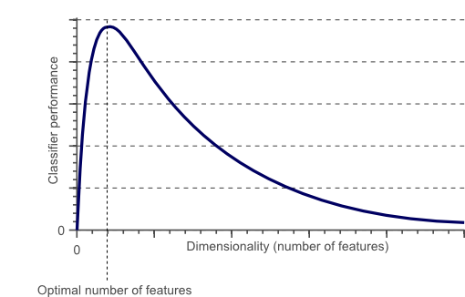
Unnecessary and redundant features not only slow down the training time of an algorithm, but they also affect the performance of the algorithm.
There are several advantages of performing feature selection before training machine learning models:
- Models with less number of features have higher explainability.
- It is easier to implement machine learning models with reduced features.
- Fewer features lead to enhanced generalization which in turn reduces overfitting.
- Feature selection removes data redundancy.
- Training time of models with fewer features is significantly lower.
- Models with fewer features are less prone to errors.
What is filter method?
Features selected using filter methods can be used as an input to any machine learning models.
- Univariate -> Fisher Score, Mutual Information Gain, Variance etc
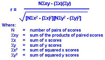
- Multi-variate -> Pearson Correlation
The univariate filter methods are the type of methods where individual features are ranked according to specific criteria. The top N features are then selected. Different types of ranking criteria are used for univariate filtermethods, for example fisher score, mutual information, and variance of the feature.
Multivariate filter methods are capable of removing redundant features from the data since they take the mutual relationship between the features into account.
Univariate Filtering Methods in this lesson
- Constant Removal
- Quasi Constant Removal
- Duplicate Feature Removal
Download Data Files
Constant Feature Removal
Importing required libraries
import numpy as np
import pandas as pd
import matplotlib.pyplot as plt
import seaborn as sns
from sklearn.model_selection import train_test_split
from sklearn.ensemble import RandomForestClassifier
from sklearn.metrics import accuracy_score
from sklearn.feature_selection import VarianceThreshold
Now read the dataset from pandas and intially number of rows are 20000.
data = pd.read_csv('santander.csv', nrows = 20000)
data.head()
| ID | var3 | var15 | imp_ent_var16_ult1 | imp_op_var39_comer_ult1 | imp_op_var39_comer_ult3 | imp_op_var40_comer_ult1 | imp_op_var40_comer_ult3 | imp_op_var40_efect_ult1 | imp_op_var40_efect_ult3 | … | saldo_medio_var33_hace2 | saldo_medio_var33_hace3 | saldo_medio_var33_ult1 | saldo_medio_var33_ult3 | saldo_medio_var44_hace2 | saldo_medio_var44_hace3 | saldo_medio_var44_ult1 | saldo_medio_var44_ult3 | var38 | TARGET | |
|---|---|---|---|---|---|---|---|---|---|---|---|---|---|---|---|---|---|---|---|---|---|
| 0 | 1 | 2 | 23 | 0.0 | 0.0 | 0.0 | 0.0 | 0.0 | 0 | 0 | … | 0.0 | 0.0 | 0.0 | 0.0 | 0.0 | 0.0 | 0.0 | 0.0 | 39205.170000 | 0 |
| 1 | 3 | 2 | 34 | 0.0 | 0.0 | 0.0 | 0.0 | 0.0 | 0 | 0 | … | 0.0 | 0.0 | 0.0 | 0.0 | 0.0 | 0.0 | 0.0 | 0.0 | 49278.030000 | 0 |
| 2 | 4 | 2 | 23 | 0.0 | 0.0 | 0.0 | 0.0 | 0.0 | 0 | 0 | … | 0.0 | 0.0 | 0.0 | 0.0 | 0.0 | 0.0 | 0.0 | 0.0 | 67333.770000 | 0 |
| 3 | 8 | 2 | 37 | 0.0 | 195.0 | 195.0 | 0.0 | 0.0 | 0 | 0 | … | 0.0 | 0.0 | 0.0 | 0.0 | 0.0 | 0.0 | 0.0 | 0.0 | 64007.970000 | 0 |
| 4 | 10 | 2 | 39 | 0.0 | 0.0 | 0.0 | 0.0 | 0.0 | 0 | 0 | … | 0.0 | 0.0 | 0.0 | 0.0 | 0.0 | 0.0 | 0.0 | 0.0 | 117310.979016 | 0 |
5 rows × 371 columns
Let’s load these datasets into x and y vectors.
X = data.drop('TARGET', axis = 1)
y = data['TARGET']
X.shape, y.shape
((20000, 370), (20000,))
Let’s split this dataset into train and test datasets using the below code.
Here test_size = 0.2 that means 20% for testing and remaining for training the model.
X_train, X_test, y_train, y_test = train_test_split(X, y, test_size = 0.2, random_state = 0, stratify = y)
Constant Features Removal
In this, first we need to create a variance threshold and then fit the model with training set of the data.
constant_filter = VarianceThreshold(threshold=0)
constant_filter.fit(X_train)
VarianceThreshold(threshold=0)
Let’s get the number of features left after removing constant features.
constant_filter.get_support().sum()
291
Let’s print the constant features list.
constant_list = [not temp for temp in constant_filter.get_support()]
constant_list
[False,
 False,
 False,
 False,
 False,
 False,
 False,
 False,
 False,
 False,
 False,
 False,
 False,
 False,
 False,
 False,
 False,
 False,
 False,
 False,
 False,
 False,
 True,
 True,
 False,
 False,
 False,
 False,
 False,
 False,
 False,
 False,
 False,
 False,
 False,
 False,
 False,
 True,
 True,
 False,
 False,
 False,
 False,
 False,
 True,
 True,
 False,
 False,
 False,
 False,
 False,
 False,
 False,
 False,
 False,
 False,
 False,
 True,
 True,
 True,
 True,
 False,
 False,
 False,
 False,
 False,
 False,
 False,
 False,
 False,
 False,
 False,
 True,
 True,
 False,
 False,
 False,
 False,
 False,
 False,
 False,
 True,
 False,
 False,
 False,
 True,
 True,
 False,
 False,
 False,
 False,
 False,
 False,
 False,
 False,
 False,
 False,
 False,
 False,
 False,
 False,
 False,
 False,
 True,
 True,
 False,
 False,
 False,
 False,
 False,
 True,
 True,
 False,
 False,
 False,
 False,
 False,
 False,
 False,
 False,
 False,
 False,
 False,
 False,
 False,
 False,
 False,
 False,
 False,
 False,
 False,
 False,
 True,
 True,
 True,
 True,
 False,
 False,
 False,
 False,
 False,
 False,
 False,
 False,
 False,
 False,
 True,
 True,
 False,
 False,
 False,
 False,
 False,
 False,
 False,
 False,
 True,
 False,
 False,
 False,
 False,
 False,
 True,
 True,
 False,
 False,
 False,
 False,
 False,
 False,
 False,
 True,
 False,
 False,
 False,
 True,
 False,
 False,
 False,
 False,
 True,
 True,
 False,
 False,
 False,
 False,
 False,
 True,
 False,
 False,
 True,
 False,
 False,
 True,
 False,
 True,
 True,
 False,
 False,
 False,
 False,
 False,
 False,
 True,
 False,
 True,
 False,
 True,
 False,
 False,
 False,
 False,
 False,
 False,
 False,
 True,
 False,
 True,
 False,
 True,
 False,
 True,
 True,
 True,
 True,
 False,
 False,
 False,
 False,
 False,
 False,
 True,
 False,
 False,
 False,
 True,
 False,
 True,
 False,
 True,
 True,
 False,
 False,
 True,
 False,
 True,
 True,
 True,
 False,
 True,
 True,
 False,
 False,
 True,
 False,
 False,
 False,
 False,
 False,
 False,
 False,
 False,
 True,
 True,
 False,
 False,
 False,
 False,
 False,
 False,
 True,
 False,
 False,
 False,
 False,
 False,
 False,
 False,
 False,
 False,
 False,
 False,
 False,
 False,
 False,
 False,
 True,
 False,
 False,
 False,
 False,
 False,
 False,
 False,
 False,
 False,
 False,
 False,
 False,
 False,
 False,
 False,
 False,
 False,
 True,
 False,
 True,
 False,
 True,
 True,
 False,
 False,
 False,
 False,
 True,
 False,
 True,
 True,
 True,
 False,
 True,
 True,
 False,
 False,
 False,
 False,
 False,
 False,
 True,
 False,
 False,
 False,
 False,
 False,
 False,
 False,
 False,
 False,
 False,
 False,
 False,
 False,
 False,
 False,
 False,
 False,
 False,
 False,
 False,
 True,
 True,
 True,
 True,
 False,
 False,
 False,
 False,
 False,
 True,
 False,
 False,
 False,
 False,
 False,
 False,
 False,
 False,
 False,
 False,
 False]
Now we will try get the name of features which are constant.
X.columns[constant_list]
Index(['ind_var2_0', 'ind_var2', 'ind_var13_medio_0', 'ind_var13_medio',
       'ind_var18_0', 'ind_var18', 'ind_var27_0', 'ind_var28_0', 'ind_var28',
       'ind_var27', 'ind_var34_0', 'ind_var34', 'ind_var41', 'ind_var46_0',
       'ind_var46', 'num_var13_medio_0', 'num_var13_medio', 'num_var18_0',
       'num_var18', 'num_var27_0', 'num_var28_0', 'num_var28', 'num_var27',
       'num_var34_0', 'num_var34', 'num_var41', 'num_var46_0', 'num_var46',
       'saldo_var13_medio', 'saldo_var18', 'saldo_var28', 'saldo_var27',
       'saldo_var34', 'saldo_var41', 'saldo_var46',
       'delta_imp_amort_var18_1y3', 'delta_imp_amort_var34_1y3',
       'delta_imp_reemb_var33_1y3', 'delta_imp_trasp_var17_out_1y3',
       'delta_imp_trasp_var33_out_1y3', 'delta_num_reemb_var33_1y3',
       'delta_num_trasp_var17_out_1y3', 'delta_num_trasp_var33_out_1y3',
       'imp_amort_var18_hace3', 'imp_amort_var18_ult1',
       'imp_amort_var34_hace3', 'imp_amort_var34_ult1', 'imp_var7_emit_ult1',
       'imp_reemb_var13_hace3', 'imp_reemb_var17_hace3',
       'imp_reemb_var33_hace3', 'imp_reemb_var33_ult1',
       'imp_trasp_var17_in_hace3', 'imp_trasp_var17_out_hace3',
       'imp_trasp_var17_out_ult1', 'imp_trasp_var33_in_hace3',
       'imp_trasp_var33_out_hace3', 'imp_trasp_var33_out_ult1',
       'ind_var7_emit_ult1', 'num_var2_0_ult1', 'num_var2_ult1',
       'num_var7_emit_ult1', 'num_meses_var13_medio_ult3',
       'num_reemb_var13_hace3', 'num_reemb_var17_hace3',
       'num_reemb_var33_hace3', 'num_reemb_var33_ult1',
       'num_trasp_var17_in_hace3', 'num_trasp_var17_out_hace3',
       'num_trasp_var17_out_ult1', 'num_trasp_var33_in_hace3',
       'num_trasp_var33_out_hace3', 'num_trasp_var33_out_ult1',
       'saldo_var2_ult1', 'saldo_medio_var13_medio_hace2',
       'saldo_medio_var13_medio_hace3', 'saldo_medio_var13_medio_ult1',
       'saldo_medio_var13_medio_ult3', 'saldo_medio_var29_hace3'],
      dtype='object')
Let’s go ahead and transform the x_train and x_test datasets into non constant datasets.
X_train_filter = constant_filter.transform(X_train)
X_test_filter = constant_filter.transform(X_test)
Let’s get the shape of the datasets.
X_train_filter.shape, X_test_filter.shape, X_train.shape
((16000, 291), (4000, 291), (16000, 370))
Quasi constant feature removal
These are the filters that are almost constant or quasi constant in other words these features have same values for large subset of outputs and such features are not very useful for making predictions.
There is no rule for fixing threshold value but generally we can take as 99% similarity and 1% of non similarity.
Let’s go ahead see how many quasi constant features are there.
quasi_constant_filter = VarianceThreshold(threshold=0.01)
quasi_constant_filter.fit(X_train_filter)
VarianceThreshold(threshold=0.01)
Let’s see how many features are non quasi constant.
quasi_constant_filter.get_support().sum()
245
291-245
46
To remove those quasi constant features, we need to apply transform on quasi transform filter object.
X_train_quasi_filter = quasi_constant_filter.transform(X_train_filter)
X_test_quasi_filter = quasi_constant_filter.transform(X_test_filter)
X_train_quasi_filter.shape, X_test_quasi_filter.shape
((16000, 245), (4000, 245))
370-245
125
In this way, we have reduced features from 370 to 245 features.
Remove Duplicate Features
If two features are exactly same those are called as duplicate features that means these features doesn’t provide any new information and makes our model complex.
Here we have a problem as we did in quasi constant and constant removal sklearn doesn’t have direct library to handle with duplicate features .
So, first we will do transpose the dataset and then python have a method to remove duplicate features.
Let’s transpose the training and testing dataset by using following code.
X_train_T = X_train_quasi_filter.T
X_test_T = X_test_quasi_filter.T
type(X_train_T)
numpy.ndarray
Let’s change into pandas dataframe.
X_train_T = pd.DataFrame(X_train_T)
X_test_T = pd.DataFrame(X_test_T)
Let’s check the shapes of the datasets.
X_train_T.shape, X_test_T.shape
((245, 16000), (245, 4000))
Let’s go ahead and get the duplicate features.
X_train_T.duplicated().sum()
18
So, here we have 18 duplicated features.
duplicated_features = X_train_T.duplicated()
duplicated_features
0      False
1      False
2      False
3      False
4      False
5      False
6      False
7      False
8      False
9      False
10     False
11     False
12     False
13     False
14     False
15     False
16     False
17     False
18     False
19     False
20     False
21     False
22     False
23     False
24     False
25     False
26     False
27     False
28     False
29     False
       ...
215    False
216    False
217    False
218    False
219    False
220    False
221    False
222    False
223    False
224    False
225    False
226    False
227    False
228    False
229    False
230    False
231    False
232    False
233    False
234    False
235    False
236    False
237    False
238    False
239    False
240    False
241    False
242    False
243    False
244    False
Length: 245, dtype: bool
Now, we need to get to non duplicated features from the following code.
features_to_keep = [not index for index in duplicated_features]
Let’s do transpose again to get the original shape.
X_train_unique = X_train_T[features_to_keep].T
X_test_unique = X_test_T[features_to_keep].T
Let’s check the shape of the datasets.
X_train_unique.shape, X_train.shape
((16000, 227), (16000, 370))
Here, we can observe original dataset has 370 features and after removal of quasi constant, constant and duplicate features we have 227 features.
370-227
143
Build ML model and compare the performance of the selected feature
Let’s go ahead and compare the model between original dataset and transformed dataset.
Here we are going to build random forest classifier.
def run_randomForest(X_train, X_test, y_train, y_test):
    clf = RandomForestClassifier(n_estimators=100, random_state=0, n_jobs=-1)
    clf.fit(X_train, y_train)
    y_pred = clf.predict(X_test)
    print('Accuracy on test set: ')
    print(accuracy_score(y_test, y_pred))
Let’s calculate the accuracy.
%%time
run_randomForest(X_train_unique, X_test_unique, y_train, y_test)
Accuracy on test set:
0.95875
Wall time: 2.18 s
Let’s check the accuracy of the original dataset.
%%time
run_randomForest(X_train, X_test, y_train, y_test)
Accuracy on test set:
0.9585
Wall time: 2.87 s
(1.51-1.26)*100/1.51
16.556291390728475
Feature Selection with Filtering Method- Correlated Feature Removal
A dataset can also contain correlated features. Two or more than two features are correlated if they are close to each other in the linear space.
Correlation between the output observations and the input features is very important and such features should be retained.
Summary
- Feature Space to target correlation is desired
- Feature to feature correlation is not desired
- If 2 features are highly correlated then either feature is redundant
- Correlation in feature space increases model complexity
- Removing correlated features improves model performance
- Different model shows different performance over the correlated features
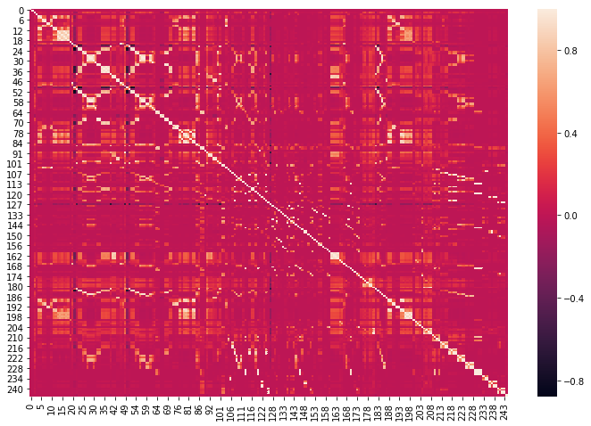
corrmat = X_train_unique.corr()
plt.figure(figsize=(12,8))
sns.heatmap(corrmat)
def get_correlation(data, threshold):
    corr_col = set()
    corrmat = data.corr()
    for i in range(len(corrmat.columns)):
        for j in range(i):
            if abs(corrmat.iloc[i, j])> threshold:
                colname = corrmat.columns[i]
                corr_col.add(colname)
    return corr_col
corr_features = get_correlation(X_train_unique, 0.85) corr_features
{5,
 7,
 9,
 11,
 12,
 14,
 15,
 16,
 17,
 18,
 23,
 24,
 28,
 29,
 30,
 32,
 33,
 35,
 36,
 38,
 42,
 46,
 47,
 50,
 51,
 52,
 53,
 54,
 55,
 56,
 57,
 58,
 60,
 61,
 62,
 65,
 67,
 68,
 69,
 70,
 72,
 76,
 80,
 81,
 82,
 83,
 84,
 86,
 87,
 88,
 91,
 93,
 95,
 98,
 100,
 101,
 103,
 104,
 111,
 115,
 117,
 120,
 121,
 125,
 136,
 138,
 143,
 146,
 149,
 153,
 154,
 157,
 158,
 161,
 162,
 163,
 164,
 169,
 170,
 173,
 180,
 182,
 183,
 184,
 185,
 188,
 189,
 190,
 191,
 192,
 193,
 194,
 195,
 197,
 198,
 199,
 204,
 205,
 207,
 208,
 215,
 216,
 217,
 219,
 220,
 221,
 223,
 224,
 227,
 228,
 229,
 230,
 231,
 232,
 234,
 235,
 236,
 237,
 238,
 239,
 240,
 241,
 242,
 243}
Let’s get the length of the correlated features.
len(corr_features)
124
Let’s drop the correlated features from the dataset.
X_train_uncorr = X_train_unique.drop(labels=corr_features, axis = 1)
X_test_uncorr = X_test_unique.drop(labels = corr_features, axis = 1)
X_train_uncorr.shape, X_test_uncorr.shape
((16000, 103), (4000, 103))
Let’s find out the accuracy and training time of the uncorrelated dataset.
%%time
run_randomForest(X_train_uncorr, X_test_uncorr, y_train, y_test)
Accuracy on test set:
0.95875
Wall time: 912 ms
Now we will find out the accuracy and training time of the original daatset.
%%time
run_randomForest(X_train, X_test, y_train, y_test)
Accuracy on test set:
0.9585
Wall time: 1.53 s
(1.53-0.912)*100/1.53
40.3921568627451
Feature Grouping and Feature Importance
corrmat
| 0 | 1 | 2 | 3 | 4 | 5 | 6 | 7 | 8 | 9 | … | 235 | 236 | 237 | 238 | 239 | 240 | 241 | 242 | 243 | 244 | |
|---|---|---|---|---|---|---|---|---|---|---|---|---|---|---|---|---|---|---|---|---|---|
| 0 | 1.000000 | -0.025277 | -0.001942 | 0.003594 | 0.004054 | -0.001697 | -0.015882 | -0.019807 | 0.000956 | -0.000588 | … | -0.001337 | 0.002051 | -0.008500 | 0.006554 | 0.005907 | 0.008825 | -0.009174 | 0.012031 | 0.012128 | 0.006612 |
| 1 | -0.025277 | 1.000000 | -0.007647 | 0.001819 | 0.008981 | 0.009232 | 0.001638 | 0.001746 | 0.000614 | 0.000695 | … | 0.000544 | 0.000586 | 0.000337 | 0.000550 | 0.000563 | 0.000922 | 0.000598 | 0.000875 | 0.000942 | 0.000415 |
| 2 | -0.001942 | -0.007647 | 1.000000 | 0.030919 | 0.106245 | 0.109140 | 0.048524 | 0.055708 | 0.004040 | 0.005796 | … | 0.025522 | 0.020168 | 0.011550 | 0.019325 | 0.019527 | 0.041321 | 0.016172 | 0.043577 | 0.044281 | -0.000810 |
| 3 | 0.003594 | 0.001819 | 0.030919 | 1.000000 | 0.029418 | 0.024905 | 0.014513 | 0.013857 | -0.000613 | -0.000691 | … | 0.014032 | -0.000583 | -0.000337 | -0.000548 | -0.000561 | 0.000541 | -0.000577 | 0.000231 | 0.000235 | 0.000966 |
| 4 | 0.004054 | 0.008981 | 0.106245 | 0.029418 | 1.000000 | 0.888789 | 0.381632 | 0.341266 | 0.012927 | 0.019674 | … | 0.002328 | 0.016743 | -0.001662 | 0.020509 | 0.021276 | -0.001905 | -0.000635 | -0.002552 | -0.002736 | 0.003656 |
| 5 | -0.001697 | 0.009232 | 0.109140 | 0.024905 | 0.888789 | 1.000000 | 0.363680 | 0.384820 | 0.017671 | 0.030060 | … | 0.000328 | 0.010860 | -0.001706 | 0.012963 | 0.013553 | 0.000871 | 0.007096 | -0.001672 | -0.001844 | 0.002257 |
| 6 | -0.015882 | 0.001638 | 0.048524 | 0.014513 | 0.381632 | 0.363680 | 1.000000 | 0.908158 | 0.030397 | 0.036359 | … | -0.000485 | 0.006351 | -0.000301 | 0.002590 | 0.003867 | -0.000818 | -0.000515 | -0.000779 | -0.000839 | 0.004448 |
| 7 | -0.019807 | 0.001746 | 0.055708 | 0.013857 | 0.341266 | 0.384820 | 0.908158 | 1.000000 | 0.047667 | 0.056456 | … | -0.000514 | 0.006336 | -0.000318 | 0.002476 | 0.003707 | -0.000866 | -0.000545 | -0.000825 | -0.000888 | 0.002427 |
| 8 | 0.000956 | 0.000614 | 0.004040 | -0.000613 | 0.012927 | 0.017671 | 0.030397 | 0.047667 | 1.000000 | 0.988256 | … | -0.000184 | -0.000197 | -0.000114 | -0.000185 | -0.000189 | -0.000309 | -0.000195 | -0.000295 | -0.000317 | -0.000739 |
| 9 | -0.000588 | 0.000695 | 0.005796 | -0.000691 | 0.019674 | 0.030060 | 0.036359 | 0.056456 | 0.988256 | 1.000000 | … | -0.000207 | -0.000222 | -0.000128 | -0.000208 | -0.000213 | -0.000349 | -0.000220 | -0.000332 | -0.000358 | -0.000811 |
| 10 | -0.012443 | 0.001517 | 0.042368 | 0.012451 | 0.298916 | 0.280081 | 0.805265 | 0.706608 | 0.388309 | 0.398826 | … | -0.000452 | -0.000485 | -0.000280 | -0.000213 | -0.000100 | -0.000762 | -0.000480 | -0.000726 | -0.000782 | 0.003341 |
| 11 | 0.010319 | 0.009097 | 0.096719 | 0.026377 | 0.938409 | 0.824893 | 0.038751 | 0.029445 | 0.002612 | 0.007677 | … | 0.002699 | 0.015727 | -0.001684 | 0.021203 | 0.021555 | -0.001754 | -0.000494 | -0.002467 | -0.002645 | 0.002290 |
| 12 | 0.005268 | 0.009360 | 0.098070 | 0.021968 | 0.838953 | 0.943622 | 0.067664 | 0.057591 | 0.002018 | 0.012266 | … | 0.000540 | 0.009474 | -0.001732 | 0.013133 | 0.013330 | 0.001253 | 0.007871 | -0.001513 | -0.001676 | 0.001570 |
| 13 | 0.017605 | -0.002511 | 0.082025 | 0.016331 | 0.266746 | 0.254702 | 0.040788 | 0.033996 | 0.108329 | 0.106806 | … | -0.001670 | 0.034002 | -0.001035 | 0.038103 | 0.038047 | 0.007400 | 0.002248 | 0.006688 | 0.006283 | 0.000707 |
| 14 | 0.016960 | -0.001086 | 0.095485 | 0.016458 | 0.326051 | 0.359897 | 0.048914 | 0.045136 | 0.081030 | 0.081962 | … | -0.002040 | 0.025566 | -0.001264 | 0.028641 | 0.028613 | 0.004485 | 0.001176 | 0.004012 | 0.003599 | -0.001992 |
| 15 | 0.018040 | 0.002426 | 0.106415 | 0.024014 | 0.638412 | 0.565620 | 0.043920 | 0.033716 | 0.083438 | 0.084688 | … | 0.000009 | 0.033265 | -0.001589 | 0.038978 | 0.039103 | 0.004773 | 0.001465 | 0.003984 | 0.003632 | 0.001339 |
| 16 | 0.017400 | -0.002401 | 0.081028 | 0.015979 | 0.263482 | 0.252160 | 0.043357 | 0.038548 | 0.214397 | 0.211633 | … | -0.001661 | 0.033386 | -0.001029 | 0.037417 | 0.037362 | 0.007237 | 0.002188 | 0.006539 | 0.006139 | 0.000614 |
| 17 | 0.016745 | -0.001019 | 0.095009 | 0.016239 | 0.324417 | 0.358769 | 0.051373 | 0.049260 | 0.160240 | 0.162113 | … | -0.002037 | 0.025295 | -0.001262 | 0.028341 | 0.028312 | 0.004412 | 0.001147 | 0.003946 | 0.003534 | -0.002038 |
| 18 | 0.015206 | 0.002629 | 0.110912 | 0.025558 | 0.673593 | 0.599584 | 0.190138 | 0.162168 | 0.152035 | 0.155173 | … | -0.000074 | 0.032155 | -0.001591 | 0.037742 | 0.037884 | 0.004487 | 0.001333 | 0.003729 | 0.003377 | 0.001910 |
| 19 | -0.000103 | 0.000519 | 0.016886 | -0.000520 | 0.049579 | 0.042621 | 0.012454 | 0.007797 | -0.000175 | -0.000198 | … | -0.000156 | -0.000167 | -0.000096 | -0.000156 | -0.000160 | -0.000262 | -0.000165 | -0.000250 | -0.000269 | 0.000213 |
| 20 | -0.001198 | 0.004590 | 0.107680 | 0.007478 | 0.227803 | 0.238159 | 0.306165 | 0.284353 | 0.125108 | 0.138077 | … | -0.001365 | -0.001462 | -0.000846 | 0.000768 | 0.001829 | 0.009008 | -0.001449 | 0.009156 | 0.011164 | -0.001227 |
| 21 | -0.006814 | -0.008975 | -0.105502 | -0.002101 | -0.208030 | -0.211873 | -0.071459 | -0.078593 | -0.012763 | -0.021318 | … | 0.002674 | -0.049920 | -0.037729 | -0.038529 | -0.041438 | -0.000421 | -0.010257 | 0.002149 | 0.002306 | -0.016447 |
| 22 | -0.002037 | 0.041015 | -0.102487 | 0.017541 | 0.041167 | 0.041372 | -0.006549 | -0.008179 | 0.003576 | 0.001088 | … | 0.009114 | -0.012641 | -0.011070 | -0.008324 | -0.009368 | 0.013263 | 0.004114 | 0.013717 | 0.014768 | -0.056029 |
| 23 | 0.010356 | 0.008019 | 0.107570 | 0.003429 | 0.200514 | 0.182937 | 0.035401 | 0.025512 | 0.012907 | 0.018006 | … | -0.002401 | 0.031418 | -0.001487 | 0.033291 | 0.034573 | 0.001397 | 0.011918 | -0.001487 | -0.001591 | 0.012346 |
| 24 | 0.012021 | 0.007439 | 0.101605 | 0.004843 | 0.220673 | 0.201909 | 0.039018 | 0.028469 | 0.014240 | 0.019760 | … | -0.002227 | 0.034079 | -0.001380 | 0.036066 | 0.037450 | 0.002086 | 0.013156 | -0.001036 | -0.001105 | -0.003767 |
| 25 | 0.001732 | 0.011525 | 0.273152 | 0.010099 | 0.027387 | 0.026378 | 0.046258 | 0.033114 | -0.003889 | -0.004384 | … | -0.003450 | 0.020817 | -0.002138 | 0.022279 | 0.023163 | -0.000543 | -0.003662 | -0.001555 | -0.001463 | 0.012034 |
| 26 | 0.001138 | 0.009467 | 0.231649 | 0.015117 | 0.033757 | 0.037053 | 0.044225 | 0.034049 | -0.003194 | -0.003600 | … | -0.002834 | 0.026148 | -0.001756 | 0.027806 | 0.028888 | 0.001500 | -0.003008 | 0.000193 | 0.000460 | 0.006643 |
| 27 | -0.004836 | 0.009771 | 0.299165 | 0.036569 | -0.010411 | -0.013701 | 0.020327 | 0.019508 | -0.003295 | -0.003715 | … | -0.002924 | -0.003132 | -0.001811 | -0.001902 | -0.001440 | -0.003893 | -0.003103 | -0.003587 | -0.003989 | 0.012240 |
| 28 | -0.006480 | 0.008796 | 0.241707 | 0.040420 | -0.012628 | -0.018755 | 0.009992 | 0.003331 | -0.002969 | -0.003347 | … | -0.002634 | -0.002822 | -0.001632 | -0.001507 | -0.000986 | -0.004438 | -0.002796 | -0.004228 | -0.004553 | 0.007400 |
| 29 | -0.005811 | 0.008676 | 0.237830 | 0.041165 | -0.012035 | -0.018146 | 0.010326 | 0.003592 | -0.002929 | -0.003301 | … | -0.002599 | -0.002784 | -0.001610 | -0.001456 | -0.000927 | -0.004378 | -0.002758 | -0.004171 | -0.004491 | 0.006121 |
| … | … | … | … | … | … | … | … | … | … | … | … | … | … | … | … | … | … | … | … | … | … |
| 215 | 0.006937 | 0.002152 | 0.043278 | 0.002314 | 0.073627 | 0.084908 | 0.009789 | 0.009653 | 0.000540 | 0.013546 | … | -0.000644 | 0.003153 | -0.000399 | 0.003511 | 0.003709 | 0.082936 | 0.230452 | 0.029915 | 0.033617 | 0.000338 |
| 216 | 0.004924 | 0.002210 | 0.045622 | 0.003234 | 0.086904 | 0.093401 | 0.042081 | 0.029906 | 0.000420 | 0.012702 | … | -0.000662 | 0.003721 | -0.000410 | 0.004129 | 0.004359 | 0.074334 | 0.206808 | 0.026758 | 0.030066 | 0.000244 |
| 217 | 0.008100 | 0.003979 | 0.149586 | 0.001554 | -0.003401 | -0.004867 | 0.024589 | 0.017603 | -0.001336 | -0.001506 | … | -0.001185 | 0.011108 | -0.000734 | 0.011385 | 0.011627 | -0.001886 | -0.001258 | -0.001828 | -0.001966 | 0.017276 |
| 218 | -0.000582 | 0.002581 | 0.093124 | -0.001262 | -0.007050 | -0.006547 | -0.002282 | -0.002111 | -0.000865 | -0.000976 | … | -0.000768 | 0.012837 | -0.000476 | 0.013076 | 0.013340 | -0.001294 | -0.000815 | -0.001232 | -0.001327 | 0.006644 |
| 219 | 0.007130 | 0.004811 | 0.178546 | 0.002540 | -0.002079 | -0.004782 | 0.036168 | 0.025934 | -0.001618 | -0.001823 | … | -0.001435 | 0.010157 | -0.000889 | 0.010430 | 0.010646 | -0.002222 | -0.001523 | -0.002103 | -0.002237 | 0.018092 |
| 220 | 0.007675 | 0.004879 | 0.179565 | 0.002948 | -0.001151 | -0.003808 | 0.038964 | 0.028107 | -0.001640 | -0.001849 | … | -0.001455 | 0.009732 | -0.000902 | 0.010011 | 0.010224 | -0.002257 | -0.001545 | -0.002116 | -0.002243 | 0.017579 |
| 221 | -0.006477 | 0.005759 | 0.178263 | -0.005438 | 0.002963 | -0.001631 | 0.048470 | 0.029154 | -0.001943 | -0.002190 | … | -0.001724 | -0.001846 | -0.001068 | -0.001729 | -0.001768 | -0.002904 | -0.001829 | -0.002766 | -0.002979 | 0.014736 |
| 222 | -0.010219 | 0.003183 | 0.094741 | -0.003083 | 0.040691 | 0.027749 | 0.133603 | 0.084716 | -0.001073 | -0.001210 | … | -0.000952 | -0.001020 | -0.000590 | -0.000958 | -0.000981 | -0.001604 | -0.001011 | -0.001528 | -0.001646 | 0.002052 |
| 223 | -0.011386 | 0.006355 | 0.200415 | 0.025778 | -0.000914 | -0.005809 | 0.038767 | 0.022672 | -0.002144 | -0.002417 | … | -0.001903 | -0.002038 | -0.001179 | -0.001788 | -0.001769 | -0.003205 | -0.002019 | -0.003054 | -0.003288 | 0.014980 |
| 224 | -0.011200 | 0.006248 | 0.195652 | 0.033042 | -0.000322 | -0.005729 | 0.043137 | 0.025504 | -0.002108 | -0.002376 | … | -0.001871 | -0.002004 | -0.001159 | -0.001801 | -0.001804 | -0.003151 | -0.001985 | -0.003002 | -0.003233 | 0.014628 |
| 225 | 0.006455 | 0.002629 | 0.125618 | -0.001532 | 0.003267 | 0.004018 | 0.013532 | 0.021485 | -0.000883 | -0.000995 | … | -0.000783 | -0.000839 | -0.000485 | -0.000788 | -0.000807 | -0.001195 | -0.000831 | -0.001146 | -0.001241 | 0.014567 |
| 226 | 0.008361 | 0.001482 | 0.059293 | 0.000238 | 0.012429 | 0.010896 | 0.001034 | 0.002878 | -0.000492 | -0.000555 | … | -0.000437 | -0.000468 | -0.000271 | -0.000439 | -0.000450 | -0.000573 | -0.000463 | -0.000556 | -0.000608 | 0.005688 |
| 227 | 0.003765 | 0.002827 | 0.135362 | -0.001817 | 0.000824 | 0.001493 | 0.012108 | 0.019415 | -0.000950 | -0.001071 | … | -0.000843 | -0.000903 | -0.000522 | -0.000848 | -0.000868 | -0.001417 | -0.000895 | -0.001348 | -0.001452 | 0.015351 |
| 228 | 0.005352 | 0.002770 | 0.132537 | -0.001698 | 0.001272 | 0.001627 | 0.010082 | 0.016429 | -0.000930 | -0.001048 | … | -0.000825 | -0.000884 | -0.000511 | -0.000830 | -0.000850 | -0.001387 | -0.000876 | -0.001318 | -0.001421 | 0.014485 |
| 229 | 0.008042 | 0.000356 | 0.023435 | -0.000354 | -0.001629 | -0.001719 | -0.000318 | -0.000337 | -0.000120 | -0.000136 | … | -0.000107 | 0.002856 | -0.000066 | 0.004306 | 0.004022 | 0.000265 | -0.000113 | 0.000089 | 0.000121 | 0.013197 |
| 230 | 0.007870 | 0.000338 | 0.022679 | -0.000338 | -0.001669 | -0.001713 | -0.000302 | -0.000320 | -0.000114 | -0.000129 | … | -0.000101 | -0.000108 | -0.000063 | -0.000102 | -0.000104 | -0.000171 | -0.000107 | -0.000163 | -0.000175 | 0.012842 |
| 231 | 0.007952 | 0.000411 | 0.025362 | -0.000285 | -0.001677 | -0.001846 | -0.000365 | -0.000387 | -0.000138 | -0.000156 | … | -0.000123 | 0.007701 | -0.000076 | 0.011513 | 0.010768 | 0.001004 | -0.000130 | 0.000510 | 0.000619 | 0.013321 |
| 232 | 0.008021 | 0.000408 | 0.025406 | -0.000334 | -0.001730 | -0.001875 | -0.000362 | -0.000383 | -0.000137 | -0.000154 | … | -0.000121 | 0.006078 | -0.000075 | 0.009101 | 0.008510 | 0.000746 | -0.000129 | 0.000360 | 0.000443 | 0.013418 |
| 233 | -0.001596 | 0.000391 | 0.013612 | -0.000391 | -0.001930 | -0.001981 | -0.000349 | -0.000370 | -0.000132 | -0.000149 | … | 0.538270 | -0.000125 | -0.000073 | -0.000118 | -0.000121 | 0.031970 | -0.000124 | 0.068648 | 0.057673 | -0.000203 |
| 234 | 0.001830 | 0.000453 | 0.023446 | 0.008469 | 0.000833 | -0.000407 | -0.000404 | -0.000428 | -0.000153 | -0.000172 | … | 0.950232 | -0.000145 | -0.000084 | -0.000136 | -0.000140 | 0.004649 | -0.000144 | 0.010219 | 0.008541 | -0.003446 |
| 235 | -0.001337 | 0.000544 | 0.025522 | 0.014032 | 0.002328 | 0.000328 | -0.000485 | -0.000514 | -0.000184 | -0.000207 | … | 1.000000 | -0.000174 | -0.000101 | -0.000164 | -0.000168 | 0.012705 | -0.000173 | 0.027515 | 0.023072 | -0.003399 |
| 236 | 0.002051 | 0.000586 | 0.020168 | -0.000583 | 0.016743 | 0.010860 | 0.006351 | 0.006336 | -0.000197 | -0.000222 | … | -0.000174 | 1.000000 | 0.484331 | 0.938668 | 0.953411 | 0.021540 | -0.000185 | 0.012393 | 0.014523 | -0.000773 |
| 237 | -0.008500 | 0.000337 | 0.011550 | -0.000337 | -0.001662 | -0.001706 | -0.000301 | -0.000318 | -0.000114 | -0.000128 | … | -0.000101 | 0.484331 | 1.000000 | 0.193281 | 0.225912 | -0.000170 | -0.000107 | -0.000162 | -0.000174 | -0.000402 |
| 238 | 0.006554 | 0.000550 | 0.019325 | -0.000548 | 0.020509 | 0.012963 | 0.002590 | 0.002476 | -0.000185 | -0.000208 | … | -0.000164 | 0.938668 | 0.193281 | 1.000000 | 0.998497 | 0.032162 | -0.000174 | 0.018565 | 0.021742 | -0.000525 |
| 239 | 0.005907 | 0.000563 | 0.019527 | -0.000561 | 0.021276 | 0.013553 | 0.003867 | 0.003707 | -0.000189 | -0.000213 | … | -0.000168 | 0.953411 | 0.225912 | 0.998497 | 1.000000 | 0.030087 | -0.000178 | 0.017358 | 0.020331 | -0.000589 |
| 240 | 0.008825 | 0.000922 | 0.041321 | 0.000541 | -0.001905 | 0.000871 | -0.000818 | -0.000866 | -0.000309 | -0.000349 | … | 0.012705 | 0.021540 | -0.000170 | 0.032162 | 0.030087 | 1.000000 | 0.329805 | 0.935317 | 0.919036 | 0.011106 |
| 241 | -0.009174 | 0.000598 | 0.016172 | -0.000577 | -0.000635 | 0.007096 | -0.000515 | -0.000545 | -0.000195 | -0.000220 | … | -0.000173 | -0.000185 | -0.000107 | -0.000174 | -0.000178 | 0.329805 | 1.000000 | 0.127224 | 0.140902 | 0.011807 |
| 242 | 0.012031 | 0.000875 | 0.043577 | 0.000231 | -0.002552 | -0.001672 | -0.000779 | -0.000825 | -0.000295 | -0.000332 | … | 0.027515 | 0.012393 | -0.000162 | 0.018565 | 0.017358 | 0.935317 | 0.127224 | 1.000000 | 0.993536 | 0.008604 |
| 243 | 0.012128 | 0.000942 | 0.044281 | 0.000235 | -0.002736 | -0.001844 | -0.000839 | -0.000888 | -0.000317 | -0.000358 | … | 0.023072 | 0.014523 | -0.000174 | 0.021742 | 0.020331 | 0.919036 | 0.140902 | 0.993536 | 1.000000 | 0.009136 |
| 244 | 0.006612 | 0.000415 | -0.000810 | 0.000966 | 0.003656 | 0.002257 | 0.004448 | 0.002427 | -0.000739 | -0.000811 | … | -0.003399 | -0.000773 | -0.000402 | -0.000525 | -0.000589 | 0.011106 | 0.011807 | 0.008604 | 0.009136 | 1.000000 |
227 rows × 227 columns
Let’s get the list of correlated features from the data.
corrdata = corrmat.abs().stack()
corrdata
0    0      1.000000
     1      0.025277
     2      0.001942
     3      0.003594
     4      0.004054
     5      0.001697
     6      0.015882
     7      0.019807
     8      0.000956
     9      0.000588
     10     0.012443
     11     0.010319
     12     0.005268
     13     0.017605
     14     0.016960
     15     0.018040
     16     0.017400
     17     0.016745
     18     0.015206
     19     0.000103
     20     0.001198
     21     0.006814
     22     0.002037
     23     0.010356
     24     0.012021
     25     0.001732
     26     0.001138
     27     0.004836
     28     0.006480
     29     0.005811
              ...
244  215    0.000338
     216    0.000244
     217    0.017276
     218    0.006644
     219    0.018092
     220    0.017579
     221    0.014736
     222    0.002052
     223    0.014980
     224    0.014628
     225    0.014567
     226    0.005688
     227    0.015351
     228    0.014485
     229    0.013197
     230    0.012842
     231    0.013321
     232    0.013418
     233    0.000203
     234    0.003446
     235    0.003399
     236    0.000773
     237    0.000402
     238    0.000525
     239    0.000589
     240    0.011106
     241    0.011807
     242    0.008604
     243    0.009136
     244    1.000000
Length: 51529, dtype: float64
Let’s arrange the correlated data in the descending order.
corrdata = corrdata.sort_values(ascending=False)
corrdata
29   58     1.000000e+00
58   29     1.000000e+00
134  158    1.000000e+00
158  134    1.000000e+00
182  182    1.000000e+00
181  181    1.000000e+00
159  159    1.000000e+00
160  160    1.000000e+00
161  161    1.000000e+00
162  162    1.000000e+00
163  163    1.000000e+00
164  164    1.000000e+00
165  165    1.000000e+00
166  166    1.000000e+00
167  167    1.000000e+00
168  168    1.000000e+00
169  169    1.000000e+00
170  170    1.000000e+00
171  171    1.000000e+00
158  158    1.000000e+00
173  173    1.000000e+00
174  174    1.000000e+00
175  175    1.000000e+00
176  176    1.000000e+00
177  177    1.000000e+00
183  183    1.000000e+00
178  178    1.000000e+00
179  179    1.000000e+00
180  180    1.000000e+00
172  172    1.000000e+00
                ...
113  60     8.925381e-06
60   113    8.925381e-06
82   193    8.892757e-06
193  82     8.892757e-06
230  110    8.848510e-06
110  230    8.848510e-06
235  15     8.707147e-06
15   235    8.707147e-06
186  243    7.715459e-06
243  186    7.715459e-06
150  120    7.232908e-06
120  150    7.232908e-06
103  189    5.738723e-06
189  103    5.738723e-06
13   120    5.200500e-06
120  13     5.200500e-06
243  162    3.905074e-06
162  243    3.905074e-06
186  126    3.594093e-06
126  186    3.594093e-06
159  242    2.877380e-06
242  159    2.877380e-06
107  68     2.392837e-06
68   107    2.392837e-06
111  229    1.934954e-06
229  111    1.934954e-06
231  150    6.044672e-07
150  231    6.044672e-07
231  123    3.966696e-07
123  231    3.966696e-07
Length: 51529, dtype: float64
Let’s get the correlated data between 1 and 0.85.
corrdata = corrdata[corrdata>0.85]
corrdata = corrdata[corrdata<1]
corrdata
143  135    1.000000
135  143    1.000000
136  128    1.000000
128  136    1.000000
31   62     1.000000
62   31     1.000000
20   47     1.000000
47   20     1.000000
52   23     1.000000
23   52     1.000000
53   24     1.000000
24   53     1.000000
33   69     1.000000
69   33     1.000000
157  133    1.000000
133  157    1.000000
237  149    1.000000
149  237    1.000000
154  132    1.000000
132  154    1.000000
146  230    0.999997
230  146    0.999997
238  122    0.999945
122  238    0.999945
148  149    0.999929
149  148    0.999929
237  148    0.999929
148  237    0.999929
231  232    0.999892
232  231    0.999892
              ...
183  52     0.860163
52   183    0.860163
183  23     0.860163
23   183    0.860163
79   195    0.859806
195  79     0.859806
8    193    0.859270
193  8      0.859270
29   61     0.858830
61   29     0.858830
     58     0.858830
58   61     0.858830
84   77     0.858529
77   84     0.858529
83   189    0.858484
189  83     0.858484
84   194    0.857731
194  84     0.857731
76   190    0.857717
190  76     0.857717
151  173    0.854991
173  151    0.854991
41   163    0.852233
163  41     0.852233
66   67     0.851384
67   66     0.851384
61   28     0.851022
28   61     0.851022
72   35     0.850893
35   72     0.850893
Length: 534, dtype: float64
corrdata = pd.DataFrame(corrdata).reset_index() corrdata.columns = ['features1', 'features2', 'corr_value'] corrdata
| features1 | features2 | corr_value | |
|---|---|---|---|
| 0 | 143 | 135 | 1.000000 |
| 1 | 135 | 143 | 1.000000 |
| 2 | 136 | 128 | 1.000000 |
| 3 | 128 | 136 | 1.000000 |
| 4 | 31 | 62 | 1.000000 |
| 5 | 62 | 31 | 1.000000 |
| 6 | 20 | 47 | 1.000000 |
| 7 | 47 | 20 | 1.000000 |
| 8 | 52 | 23 | 1.000000 |
| 9 | 23 | 52 | 1.000000 |
| 10 | 53 | 24 | 1.000000 |
| 11 | 24 | 53 | 1.000000 |
| 12 | 33 | 69 | 1.000000 |
| 13 | 69 | 33 | 1.000000 |
| 14 | 157 | 133 | 1.000000 |
| 15 | 133 | 157 | 1.000000 |
| 16 | 237 | 149 | 1.000000 |
| 17 | 149 | 237 | 1.000000 |
| 18 | 154 | 132 | 1.000000 |
| 19 | 132 | 154 | 1.000000 |
| 20 | 146 | 230 | 0.999997 |
| 21 | 230 | 146 | 0.999997 |
| 22 | 238 | 122 | 0.999945 |
| 23 | 122 | 238 | 0.999945 |
| 24 | 148 | 149 | 0.999929 |
| 25 | 149 | 148 | 0.999929 |
| 26 | 237 | 148 | 0.999929 |
| 27 | 148 | 237 | 0.999929 |
| 28 | 231 | 232 | 0.999892 |
| 29 | 232 | 231 | 0.999892 |
| … | … | … | … |
| 504 | 183 | 52 | 0.860163 |
| 505 | 52 | 183 | 0.860163 |
| 506 | 183 | 23 | 0.860163 |
| 507 | 23 | 183 | 0.860163 |
| 508 | 79 | 195 | 0.859806 |
| 509 | 195 | 79 | 0.859806 |
| 510 | 8 | 193 | 0.859270 |
| 511 | 193 | 8 | 0.859270 |
| 512 | 29 | 61 | 0.858830 |
| 513 | 61 | 29 | 0.858830 |
| 514 | 61 | 58 | 0.858830 |
| 515 | 58 | 61 | 0.858830 |
| 516 | 84 | 77 | 0.858529 |
| 517 | 77 | 84 | 0.858529 |
| 518 | 83 | 189 | 0.858484 |
| 519 | 189 | 83 | 0.858484 |
| 520 | 84 | 194 | 0.857731 |
| 521 | 194 | 84 | 0.857731 |
| 522 | 76 | 190 | 0.857717 |
| 523 | 190 | 76 | 0.857717 |
| 524 | 151 | 173 | 0.854991 |
| 525 | 173 | 151 | 0.854991 |
| 526 | 41 | 163 | 0.852233 |
| 527 | 163 | 41 | 0.852233 |
| 528 | 66 | 67 | 0.851384 |
| 529 | 67 | 66 | 0.851384 |
| 530 | 61 | 28 | 0.851022 |
| 531 | 28 | 61 | 0.851022 |
| 532 | 72 | 35 | 0.850893 |
| 533 | 35 | 72 | 0.850893 |
534 rows × 3 columns
Let’s have a list of uncorrelated features from the dataset.
grouped_feature_list = []
correlated_groups_list = []
for feature in corrdata.features1.unique():
    if feature not in grouped_feature_list:
        correlated_block = corrdata[corrdata.features1 == feature]
        grouped_feature_list = grouped_feature_list + list(correlated_block.features2.unique()) + [feature]
        correlated_groups_list.append(correlated_block)
len(correlated_groups_list)
56
X_train.shape, X_train_uncorr.shape
((16000, 370), (16000, 103))
for group in correlated_groups_list:
    print(group)
   features1  features2  corr_value
0        143        135         1.0
     features1  features2  corr_value
2          136        128    1.000000
197        136        169    0.959468
   features1  features2  corr_value
4         31         62         1.0
   features1  features2  corr_value
6         20         47         1.0
     features1  features2  corr_value
8           52         23    1.000000
297         52         24    0.927683
299         52         53    0.927683
448         52         21    0.877297
505         52        183    0.860163
     features1  features2  corr_value
12          33         69    1.000000
224         33         32    0.947113
228         33         68    0.946571
322         33         26    0.917665
337         33         55    0.914178
422         33        184    0.884383
    features1  features2  corr_value
14        157        133         1.0
    features1  features2  corr_value
16        237        149    1.000000
26        237        148    0.999929
    features1  features2  corr_value
18        154        132         1.0
     features1  features2  corr_value
20         146        230    0.999997
36         146        229    0.999778
59         146        231    0.997052
68         146        232    0.996772
76         146        113    0.996424
89         146        120    0.993307
245        146        170    0.944314
     features1  features2  corr_value
22         238        122    0.999945
49         238        239    0.998497
264        238        236    0.938668
    features1  features2  corr_value
34         82         78    0.999859
     features1  features2  corr_value
40         108        115    0.999478
97         108        219    0.992870
115        108        125    0.987333
142        108        220    0.982474
280        108        217    0.933815
     features1  features2  corr_value
46         199        197    0.998753
362        199        196    0.905699
371        199        198    0.904341
     features1  features2  corr_value
50         181        208    0.997718
345        181        205    0.911453
467        181        207    0.871801
     features1  features2  corr_value
72          17         14    0.996739
396         17         16    0.890442
408         17         13    0.888669
     features1  features2  corr_value
86         242        243    0.993536
122        242        126    0.986744
276        242        240    0.935317
     features1  features2  corr_value
92          28         57    0.993186
124         28         58    0.986371
126         28         29    0.986371
185         28        185    0.964067
381         28         27    0.901032
399         28         30    0.889321
531         28         61    0.851022
     features1  features2  corr_value
94          51         22    0.992882
385         51        182    0.899063
     features1  features2  corr_value
100         44         46    0.990593
377         44         98    0.902736
410         44         95    0.888337
     features1  features2  corr_value
102         77         81    0.989793
461         77         80    0.874240
517         77         84    0.858529
     features1  features2  corr_value
104        109        223    0.989341
151        109        224    0.980951
356        109        221    0.907987
413        109        111    0.887721
     features1  features2  corr_value
112          9          8    0.988256
417          9        193    0.886955
444          9        192    0.878045
     features1  features2  corr_value
116        227        228    0.987304
188        227        225    0.962657
     features1  features2  corr_value
118        116        117    0.987013
     features1  features2  corr_value
128         91         49    0.985951
     features1  features2  corr_value
130         54         25    0.985875
419         54        100    0.886309
     features1  features2  corr_value
134         76         75    0.984751
353         76         74    0.908497
477         76        191    0.870551
522         76        190    0.857717
     features1  features2  corr_value
136         38         35    0.984077
261         38         34    0.940390
306         38         36    0.922699
496         38         72    0.864661
     features1  features2  corr_value
138         18         15    0.983164
465         18         16    0.872133
470         18         13    0.870936
     features1  features2  corr_value
140        215        107    0.983156
146        215        216    0.981815
     features1  features2  corr_value
161         56         61    0.976942
187         56         27    0.962726
211         56         30    0.953194
     features1  features2  corr_value
164        162        163    0.975002
288        162        161    0.930635
369        162        164    0.904702
463        162         41    0.874083
     features1  features2  corr_value
166        102        103    0.974341
     features1  features2  corr_value
168         83         79    0.973140
263         83        188    0.938960
273         83         84    0.936080
315         83        194    0.919405
351         83         80    0.910385
518         83        189    0.858484
     features1  features2  corr_value
174         70         72    0.972088
500         70         35    0.862850
     features1  features2  corr_value
180         59         60    0.968504
     features1  features2  corr_value
207        195        189    0.956666
313        195         80    0.920961
330        195        194    0.916442
378        195         84    0.902276
428        195        188    0.882312
509        195         79    0.859806
     features1  features2  corr_value
216        235        234    0.950232
349        235        106    0.911179
     features1  features2  corr_value
220         10        104    0.948845
     features1  features2  corr_value
234        180        179    0.945288
     features1  features2  corr_value
236        241        151    0.944812
     features1  features2  corr_value
243         42         41    0.944451
415         42        161    0.887059
503         42        164    0.861507
     features1  features2  corr_value
248         12          5    0.943622
434         12         11    0.881673
     features1  features2  corr_value
266          4         11    0.938409
402          4          5    0.888789
     features1  features2  corr_value
274         93         92    0.935867
     features1  features2  corr_value
290         89        121    0.928898
     features1  features2  corr_value
304         88         87       0.924
     features1  features2  corr_value
318        174        204    0.918533
     features1  features2  corr_value
333         50         21    0.916137
     features1  features2  corr_value
354          6          7    0.908158
     features1  features2  corr_value
372         64         65    0.904095
488         64         87    0.866430
     features1  features2  corr_value
374        101         86    0.903641
394        101         40    0.892951
     features1  features2  corr_value
390        131        153     0.89633
     features1  features2  corr_value
525        173        151    0.854991
     features1  features2  corr_value
528         66         67    0.851384
Feature Importance based on tree based classifiers
Let’s get the list of important features from the following code.
important_features = []
for group in correlated_groups_list:
    features = list(group.features1.unique()) + list(group.features2.unique())
    rf = RandomForestClassifier(n_estimators=100, random_state=0)
    rf.fit(X_train_unique[features], y_train)

    importance = pd.concat([pd.Series(features), pd.Series(rf.feature_importances_)], axis = 1)
    importance.columns = ['features', 'importance']
    importance.sort_values(by = 'importance', ascending = False, inplace = True)
    feat = importance.iloc[0]
    important_features.append(feat)
important_features
[features      135.00
 importance      0.51
 Name: 1, dtype: float64, features      128.000000
 importance      0.563757
 Name: 1, dtype: float64, features      62.00
 importance     0.51
 Name: 1, dtype: float64, features      47.00
 importance     0.51
 Name: 1, dtype: float64, features      183.000000
 importance      0.285817
 Name: 5, dtype: float64, features      184.00000
 importance      0.34728
 Name: 6, dtype: float64, features      157.00
 importance      0.34
 Name: 0, dtype: float64, features      148.000000
 importance      0.505844
 Name: 2, dtype: float64, features      132.00
 importance      0.39
 Name: 1, dtype: float64, features      120.000000
 importance      0.749683
 Name: 6, dtype: float64, features      122.00
 importance      0.34
 Name: 1, dtype: float64, features      82.000000
 importance     0.518827
 Name: 0, dtype: float64, features      125.000000
 importance      0.940524
 Name: 3, dtype: float64, features      197.000000
 importance      0.289727
 Name: 1, dtype: float64, features      207.000000
 importance      0.312834
 Name: 3, dtype: float64, features      17.000000
 importance     0.286833
 Name: 0, dtype: float64, features      243.000000
 importance      0.431557
 Name: 1, dtype: float64, features      185.000000
 importance      0.391367
 Name: 4, dtype: float64, features      182.000000
 importance      0.432045
 Name: 2, dtype: float64, features      95.000000
 importance     0.487162
 Name: 3, dtype: float64, features      84.000000
 importance     0.299008
 Name: 3, dtype: float64, features      221.00000
 importance      0.28555
 Name: 3, dtype: float64, features      8.000000
 importance    0.345509
 Name: 1, dtype: float64, features      228.000000
 importance      0.434186
 Name: 1, dtype: float64, features      117.000000
 importance      0.517013
 Name: 1, dtype: float64, features      49.000000
 importance     0.500161
 Name: 1, dtype: float64, features      100.000000
 importance      0.386775
 Name: 2, dtype: float64, features      191.000000
 importance      0.345104
 Name: 3, dtype: float64, features      34.000000
 importance     0.283901
 Name: 2, dtype: float64, features      15.000000
 importance     0.400677
 Name: 1, dtype: float64, features      107.000000
 importance      0.349126
 Name: 1, dtype: float64, features      61.000000
 importance     0.323735
 Name: 1, dtype: float64, features      41.000000
 importance     0.386338
 Name: 4, dtype: float64, features      102.000000
 importance      0.508955
 Name: 0, dtype: float64, features      189.000000
 importance      0.229269
 Name: 6, dtype: float64, features      72.000000
 importance     0.490102
 Name: 1, dtype: float64, features      60.00000
 importance     0.50052
 Name: 1, dtype: float64, features      79.000000
 importance     0.213903
 Name: 6, dtype: float64, features      234.000000
 importance      0.445719
 Name: 1, dtype: float64, features      104.000000
 importance      0.640915
 Name: 1, dtype: float64, features      179.000000
 importance      0.634779
 Name: 1, dtype: float64, features      151.00
 importance      0.51
 Name: 1, dtype: float64, features      161.000000
 importance      0.346426
 Name: 2, dtype: float64, features      5.000000
 importance    0.356386
 Name: 1, dtype: float64, features      5.000000
 importance    0.403831
 Name: 2, dtype: float64, features      93.000000
 importance     0.544349
 Name: 0, dtype: float64, features      121.00
 importance      0.51
 Name: 1, dtype: float64, features      87.000000
 importance     0.553622
 Name: 1, dtype: float64, features      174.000000
 importance      0.743723
 Name: 0, dtype: float64, features      50.000000
 importance     0.616659
 Name: 0, dtype: float64, features      7.000000
 importance    0.545702
 Name: 1, dtype: float64, features      87.0000
 importance     0.7462
 Name: 2, dtype: float64, features      86.000000
 importance     0.447693
 Name: 1, dtype: float64, features      153.00
 importance      0.51
 Name: 1, dtype: float64, features      151.00
 importance      0.51
 Name: 1, dtype: float64, features      66.000000
 importance     0.630293
 Name: 0, dtype: float64]
important_features = pd.DataFrame(important_features)
important_features.reset_index(inplace=True, drop = True)
important_features
| features | importance | |
|---|---|---|
| 0 | 135.0 | 0.510000 |
| 1 | 128.0 | 0.563757 |
| 2 | 62.0 | 0.510000 |
| 3 | 47.0 | 0.510000 |
| 4 | 183.0 | 0.285817 |
| 5 | 184.0 | 0.347280 |
| 6 | 157.0 | 0.340000 |
| 7 | 148.0 | 0.505844 |
| 8 | 132.0 | 0.390000 |
| 9 | 120.0 | 0.749683 |
| 10 | 122.0 | 0.340000 |
| 11 | 82.0 | 0.518827 |
| 12 | 125.0 | 0.940524 |
| 13 | 197.0 | 0.289727 |
| 14 | 207.0 | 0.312834 |
| 15 | 17.0 | 0.286833 |
| 16 | 243.0 | 0.431557 |
| 17 | 185.0 | 0.391367 |
| 18 | 182.0 | 0.432045 |
| 19 | 95.0 | 0.487162 |
| 20 | 84.0 | 0.299008 |
| 21 | 221.0 | 0.285550 |
| 22 | 8.0 | 0.345509 |
| 23 | 228.0 | 0.434186 |
| 24 | 117.0 | 0.517013 |
| 25 | 49.0 | 0.500161 |
| 26 | 100.0 | 0.386775 |
| 27 | 191.0 | 0.345104 |
| 28 | 34.0 | 0.283901 |
| 29 | 15.0 | 0.400677 |
| 30 | 107.0 | 0.349126 |
| 31 | 61.0 | 0.323735 |
| 32 | 41.0 | 0.386338 |
| 33 | 102.0 | 0.508955 |
| 34 | 189.0 | 0.229269 |
| 35 | 72.0 | 0.490102 |
| 36 | 60.0 | 0.500520 |
| 37 | 79.0 | 0.213903 |
| 38 | 234.0 | 0.445719 |
| 39 | 104.0 | 0.640915 |
| 40 | 179.0 | 0.634779 |
| 41 | 151.0 | 0.510000 |
| 42 | 161.0 | 0.346426 |
| 43 | 5.0 | 0.356386 |
| 44 | 5.0 | 0.403831 |
| 45 | 93.0 | 0.544349 |
| 46 | 121.0 | 0.510000 |
| 47 | 87.0 | 0.553622 |
| 48 | 174.0 | 0.743723 |
| 49 | 50.0 | 0.616659 |
| 50 | 7.0 | 0.545702 |
| 51 | 87.0 | 0.746200 |
| 52 | 86.0 | 0.447693 |
| 53 | 153.0 | 0.510000 |
| 54 | 151.0 | 0.510000 |
| 55 | 66.0 | 0.630293 |
Let’s get the features which are to be discarded.
features_to_consider = set(important_features['features'])
features_to_discard = set(corr_features) - set(features_to_consider)
features_to_discard = list(features_to_discard)
X_train_grouped_uncorr = X_train_unique.drop(labels = features_to_discard, axis = 1)
Let’s get the shape of the uncorrelated dataset.
X_train_grouped_uncorr.shape
(16000, 140)
X_test_grouped_uncorr = X_test_unique.drop(labels=features_to_discard, axis = 1)
X_test_grouped_uncorr.shape
(4000, 140)
%%time
run_randomForest(X_train_grouped_uncorr, X_test_grouped_uncorr, y_train, y_test)
Accuracy on test set:
0.95775
Wall time: 1.01 s
%%time
run_randomForest(X_train, X_test, y_train, y_test)
Accuracy on test set:
0.9585
Wall time: 1.48 s
%%time
run_randomForest(X_train_uncorr, X_test_uncorr, y_train, y_test)
Accuracy on test set:
0.95875
Wall time: 891 ms

3 Comments