Prediction of Human Activity

In this project we are going to use accelometer data to train the model so that it can predict the human activity. We are going to use 2D Convolutional Neural Networks to build the model.

source = “Deep Neural Network Example” by Nils Ackermann is licensed under Creative Commons CC BY-ND 4.0

Dataset

Dataset Link: http://www.cis.fordham.edu/wisdm/dataset.php or https://github.com/laxmimerit/Human-Activity-Recognition-Using-Accelerometer-Data-and-CNN

This WISDM dataset contains data collected through controlled, laboratory conditions. The total number of examples is 1,098,207. The dataset contains six different labels (Downstairs, Jogging, Sitting, Standing, Upstairs, Walking).

Here we are importing the necessary libraries. We will be using tensorflow-keras to build the CNN. We are also importing the necessary layers required to build the CNN.

import tensorflow as tf
from tensorflow.keras import Sequential
from tensorflow.keras.layers import Flatten, Dense, Dropout, BatchNormalization
from tensorflow.keras.layers import Conv2D, MaxPool2D
from tensorflow.keras.optimizers import Adam
print(tf.__version__)

2.1.0

• pandas is used to read the dataset.
• numpy is used to perform basic array operations.
• pyplot from matplotlib is used to visualize the results.
• train_test_split from sklearn is used split the data into training and testing dataset.
• LabelEncoder from sklearn is used to encode target labels with value between 0 and number of classes-1.
• StandardScaler from sklearn is used to bring all the data in the same scale.

import pandas as pd
import numpy as np
import matplotlib.pyplot as plt
from sklearn.model_selection import train_test_split
from sklearn.preprocessing import StandardScaler, LabelEncoder

Load and process the Dataset

If we try to read this data directly using pd.read_csv() we will get an error because this data is not pre-processed properly. So we will have to read this data into a native python file and then pre-process it.

Using open() we will first open the file. Then we will read all the lines of the file into the read variable. Now we will consider all the lines one by one using a for loop. For each line the following operations will be performed-

• line = line.split(',') splits the line wherever there is a comma and returns an array of separated elements.
• last = line[5].split(';')[0] removes the semicolon after the last element in the array.
• last = last.strip() removes any extra space.
• Then if last is not empty we copy all the elements into temp.
• Now that the line is ready we append it to processedList

try and except is used for error handling. In this process if we get an error, the number of the line which is throwing that error is displayed.

file = open('WISDM_ar_v1.1/WISDM_ar_v1.1_raw.txt')
lines = file.readlines()

processedList = []

for i, line in enumerate(lines):
    try:
        line = line.split(',')
        last = line[5].split(';')[0]
        last = last.strip()
        if last == '':
            break;
        temp = [line[0], line[1], line[2], line[3], line[4], last]
        processedList.append(temp)
    except:
        print('Error at line number: ', i)

Error at line number:  281873
Error at line number:  281874
Error at line number:  281875

Now we have the processedList. It is a list of lists. Each inner list has the user ID, activity, timestamp and then the x, y, z data.

processedList[:10]

[['33', 'Jogging', '49105962326000', '-0.6946377', '12.680544', '0.50395286'],
 ['33', 'Jogging', '49106062271000', '5.012288', '11.264028', '0.95342433'],
 ['33', 'Jogging', '49106112167000', '4.903325', '10.882658', '-0.08172209'],
 ['33', 'Jogging', '49106222305000', '-0.61291564', '18.496431', '3.0237172'],
 ['33', 'Jogging', '49106332290000', '-1.1849703', '12.108489', '7.205164'],
 ['33', 'Jogging', '49106442306000', '1.3756552', '-2.4925237', '-6.510526'],
 ['33', 'Jogging', '49106542312000', '-0.61291564', '10.56939', '5.706926'],
 ['33', 'Jogging', '49106652389000', '-0.50395286', '13.947236', '7.0553403'],
 ['33', 'Jogging', '49106762313000', '-8.430995', '11.413852', '5.134871'],
 ['33', 'Jogging', '49106872299000', '0.95342433', '1.3756552', '1.6480621']]

Now we will create a DataFrame with the processed data and proper column names. data.head() will display the first 5 rows of data.

columns = ['user', 'activity', 'time', 'x', 'y', 'z']
data = pd.DataFrame(data = processedList, columns = columns)
data.head()

	user	activity	time	x	y	z
0	33	Jogging	49105962326000	-0.6946377	12.680544	0.50395286
1	33	Jogging	49106062271000	5.012288	11.264028	0.95342433
2	33	Jogging	49106112167000	4.903325	10.882658	-0.08172209
3	33	Jogging	49106222305000	-0.61291564	18.496431	3.0237172
4	33	Jogging	49106332290000	-1.1849703	12.108489	7.205164

data has 343416 rows and 6 columns.

data.shape

(343416, 6)

This will give more information about data. It says that all the values are string objects.

data.info()

<class 'pandas.core.frame.DataFrame'>
RangeIndex: 343416 entries, 0 to 343415
Data columns (total 6 columns):
user        343416 non-null object
activity    343416 non-null object
time        343416 non-null object
x           343416 non-null object
y           343416 non-null object
z           343416 non-null object
dtypes: object(6)
memory usage: 15.7+ MB

Now we will see if any null values are present in the dataset using isnull().

data.isnull().sum()

user        0
activity    0
time        0
x           0
y           0
z           0
dtype: int64

To see the distribution of data we will see the count of each unique activity using value_counts().

data['activity'].value_counts()

Walking       137375
Jogging       129392
Upstairs       35137
Downstairs     33358
Sitting         4599
Standing        3555
Name: activity, dtype: int64

Balance this data

From the data distribution shown above we can observe that the data is unbalanced. Standing has very less examples compared to Walking and Jogging'. If we use this data directly it will overfit and will be skewed towards Walking and Jogging'.

As we saw earlier the data is in string data type. Here we have converted the x, y, z values into floating values using astype('float').

data['x'] = data['x'].astype('float')
data['y'] = data['y'].astype('float')
data['z'] = data['z'].astype('float')

We can see that the data type of x, y, z has changed.

data.info()

<class 'pandas.core.frame.DataFrame'>
RangeIndex: 343416 entries, 0 to 343415
Data columns (total 6 columns):
user        343416 non-null object
activity    343416 non-null object
time        343416 non-null object
x           343416 non-null float64
y           343416 non-null float64
z           343416 non-null float64
dtypes: float64(3), object(3)
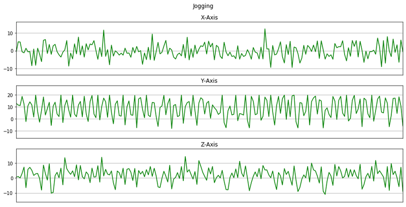
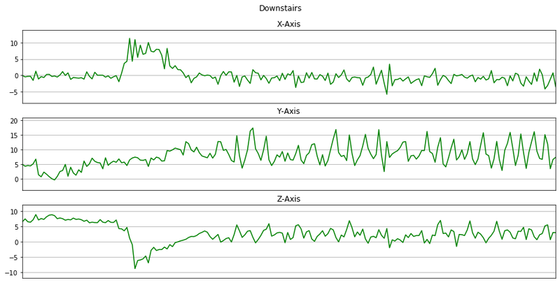
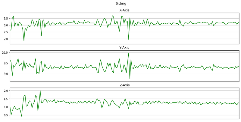
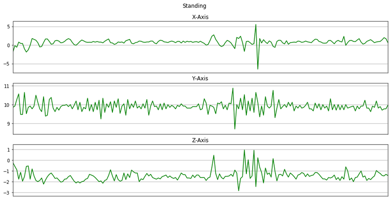
memory usage: 15.7+ MB

Now we will plot x, y, z for few seconds. The sampling rate of this data is 20Hz. So we have set a variable Fs=20. activities is a list of all the unique activities.

Fs = 20
activities = data['activity'].value_counts().index
activities

Index(['Walking', 'Jogging', 'Upstairs', 'Downstairs', 'Sitting', 'Standing'], dtype='object')

Now we will plot x, y, z for each activity for 10 seconds.

def plot_activity(activity, data):
    fig, (ax0, ax1, ax2) = plt.subplots(nrows=3, figsize=(15, 7), sharex=True)
    plot_axis(ax0, data['time'], data['x'], 'X-Axis')
    plot_axis(ax1, data['time'], data['y'], 'Y-Axis')
    plot_axis(ax2, data['time'], data['z'], 'Z-Axis')
    plt.subplots_adjust(hspace=0.2)
    fig.suptitle(activity)
    plt.subplots_adjust(top=0.90)
    plt.show()

def plot_axis(ax, x, y, title):
    ax.plot(x, y, 'g')
    ax.set_title(title)
    ax.xaxis.set_visible(False)
    ax.set_ylim([min(y) - np.std(y), max(y) + np.std(y)])
    ax.set_xlim([min(x), max(x)])
    ax.grid(True)

for activity in activities:
    data_for_plot = data[(data['activity'] == activity)][:Fs*10]
    plot_activity(activity, data_for_plot)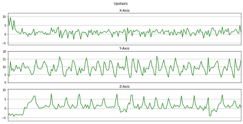

Here we will remove the columns user and time from the dataset by using drop().

df = data.drop(['user', 'time'], axis = 1).copy()
df.head()

	activity	x	y	z
0	Jogging	-0.694638	12.680544	0.503953
1	Jogging	5.012288	11.264028	0.953424
2	Jogging	4.903325	10.882658	-0.081722
3	Jogging	-0.612916	18.496431	3.023717
4	Jogging	-1.184970	12.108489	7.205164

df['activity'].value_counts()

Walking       137375
Jogging       129392
Upstairs       35137
Downstairs     33358
Sitting         4599
Standing        3555
Name: activity, dtype: int64

As this data is highly imbalanced we will take only the first 3555 lines for each activity into seperate lists. Then we will create a dataframe balanced_data using pd.DataFrame() and append all the lists to balanced_data. The final shape of balanced_data is 21330 rows and 4 columns.

Walking = df[df['activity']=='Walking'].head(3555).copy()
Jogging = df[df['activity']=='Jogging'].head(3555).copy()
Upstairs = df[df['activity']=='Upstairs'].head(3555).copy()
Downstairs = df[df['activity']=='Downstairs'].head(3555).copy()
Sitting = df[df['activity']=='Sitting'].head(3555).copy()
Standing = df[df['activity']=='Standing'].copy()

balanced_data = pd.DataFrame()
balanced_data = balanced_data.append([Walking, Jogging, Upstairs, Downstairs, Sitting, Standing])
balanced_data.shape

(21330, 4)

Now the data is balanced. We can see this by calling value_counts() on the activity column of balanced_data.

balanced_data['activity'].value_counts()

Upstairs      3555
Walking       3555
Jogging       3555
Standing      3555
Sitting       3555
Downstairs    3555
Name: activity, dtype: int64

balanced_data.head()

	activity	x	y	z
597	Walking	0.844462	8.008764	2.792171
598	Walking	1.116869	8.621680	3.786457
599	Walking	-0.503953	16.657684	1.307553
600	Walking	4.794363	10.760075	-1.184970
601	Walking	-0.040861	9.234595	-0.694638

As we can see above, the values in activity are of data type string. We will convert them into numeric values using LabelEncoder from sklearn which we have already imported. fit_tranform fits label encoder and returns encoded labels. We will add a new column in the dataset with the name label which will have the encoded values.

label = LabelEncoder()
balanced_data['label'] = label.fit_transform(balanced_data['activity'])
balanced_data.head()

	activity	x	y	z	label
597	Walking	0.844462	8.008764	2.792171	5
598	Walking	1.116869	8.621680	3.786457	5
599	Walking	-0.503953	16.657684	1.307553	5
600	Walking	4.794363	10.760075	-1.184970	5
601	Walking	-0.040861	9.234595	-0.694638	5

We can use .classes_ attribute to recover the mapping of classes.

label.classes_

array(['Downstairs', 'Jogging', 'Sitting', 'Standing', 'Upstairs',
       'Walking'], dtype=object)

Standardization of data

Here we are reading the feature space into X and the label into y.

X = balanced_data[['x', 'y', 'z']]
y = balanced_data['label']

Now we will bring all the values in X in the same range using StandardScaler() from sklearn which we have already imported. scaled_X contains the scaled values of x, y, z and the labels.

scaler = StandardScaler()
X = scaler.fit_transform(X)

scaled_X = pd.DataFrame(data = X, columns = ['x', 'y', 'z'])
scaled_X['label'] = y.values

scaled_X.head()

	x	y	z	label
0	0.000503	-0.099190	0.337933	5
1	0.073590	0.020386	0.633446	5
2	-0.361275	1.588160	-0.103312	5
3	1.060258	0.437573	-0.844119	5
4	-0.237028	0.139962	-0.698386	5

Frame Preparation

We are going to divide the data into frames of 4 seconds. To do this we will import scipy.stats.

import scipy.stats as stats

We will multiply the frequency by 4 seconds. Hence we will consider 80 observations at a time. Hop size will be 40 which means there will be some overlapping.

Fs = 20
frame_size = Fs*4 # 80
hop_size = Fs*2 # 40

get_frames() creates frames of 4 seconds i.e. 80 observations with advancement of 40 observations. The label for this 4 seconds frame is the mode of the labels for the 80 observations which make the 4 seconds frame. get_frames() returns two np.arrays: frames containing all the 4 second frames and labels containing its corresponding labels. These are stored in X and y respectively. X contains 532 frames, each having 80 values of x, y, z. y containes 532 labels for the frames in X.

def get_frames(df, frame_size, hop_size):

    N_FEATURES = 3

    frames = []
    labels = []
    for i in range(0, len(df) - frame_size, hop_size):
        x = df['x'].values[i: i + frame_size]
        y = df['y'].values[i: i + frame_size]
        z = df['z'].values[i: i + frame_size]
        
        # Retrieve the most often used label in this segment
        label = stats.mode(df['label'][i: i + frame_size])[0][0]
        frames.append([x, y, z])
        labels.append(label)

    # Bring the segments into a better shape
    frames = np.asarray(frames).reshape(-1, frame_size, N_FEATURES)
    labels = np.asarray(labels)

    return frames, labels

X, y = get_frames(scaled_X, frame_size, hop_size)

X.shape, y.shape

((532, 80, 3), (532,))

We have 3555 observations for each of the 6 activities. Hence we have a total of (3555*6) observations. This divided by the hop_size which is 40 is approximately 532. Hence we have 532 frames in our data.

(3555*6)/40

533.25

Here we are dividing the data into training data and test data using train_test_split() from sklearn which we have already imported. We are going to use 80% of the data for training the model and 20% of the data for testing. random_state controls the shuffling applied to the data before applying the split. stratify = y splits the data in a stratified fashion, using y as the class labels.

We can see that we have got 425 samples in the traning dataset and 107 samples in the test dataset.

X_train, X_test, y_train, y_test = train_test_split(X, y, test_size = 0.2, random_state = 0, stratify = y)

X_train.shape, X_test.shape

((425, 80, 3), (107, 80, 3))

The entire dataset is 3 dimentional but each sample in the data is 2 dimentional.

X_train[0].shape, X_test[0].shape

((80, 3), (80, 3))

CNN accepts 3 dimentional data so we are going to reshape() our data.

X_train = X_train.reshape(425, 80, 3, 1)
X_test = X_test.reshape(107, 80, 3, 1)

Now we can see that each sample in the dataset is 3 dimentional.

X_train[0].shape, X_test[0].shape

((80, 3, 1), (80, 3, 1))

2D CNN Model

A Sequential() model is appropriate for a plain stack of layers where each layer has exactly one input tensor and one output tensor.

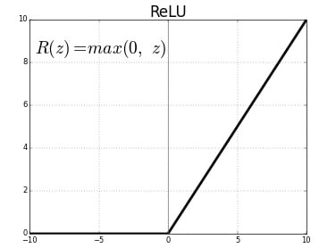
Conv2D() is a 2D Convolution Layer, this layer creates a convolution kernel that is wind with layers input which helps produce a tensor of outputs. In image processing kernel is a convolution matrix or masks which can be used for blurring, sharpening, embossing, edge detection, and more by doing a convolution between a kernel and an image. In the first Conv2D() layer we are learning a total of 16 filters each having size (2,2). We will be using ReLu activation function. The rectified linear activation function or ReLU for short is a piecewise linear function that will output the input directly if it is positive, otherwise, it will output zero.

Dropout layer is used to by randomly set the outgoing edges of hidden units to 0 at each update of the training phase. The value passed in dropout specifies the probability at which outputs of the layer are dropped out.

Flatten() is used to convert the data into a 1-dimensional array for inputting it to the next layer.

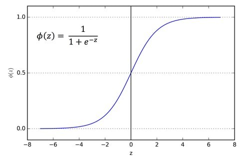
Dense layer is the regular deeply connected neural network layer with 64 neurons. The output layer is also a dense layer with 6 neurons for the 6 classes. The activation function used is softmax. Softmax converts a real vector to a vector of categorical probabilities. The elements of the output vector are in range (0, 1) and sum to 1. Softmax is often used as the activation for the last layer of a classification network because the result could be interpreted as a probability distribution.

model = Sequential()
model.add(Conv2D(16, (2, 2), activation = 'relu', input_shape = X_train[0].shape))
model.add(Dropout(0.1))

model.add(Conv2D(32, (2, 2), activation='relu'))
model.add(Dropout(0.2))

model.add(Flatten())

model.add(Dense(64, activation = 'relu'))
model.add(Dropout(0.5))

model.add(Dense(6, activation='softmax'))

Here we are compiling the model and fitting it to the training data. We will use 10 epochs to train the model. An epoch is an iteration over the entire data provided. validation_data is the data on which to evaluate the loss and any model metrics at the end of each epoch. The model will not be trained on this data. As metrics = ['accuracy'] the model will be evaluated based on the accuracy.

model.compile(optimizer=Adam(learning_rate = 0.001), loss = 'sparse_categorical_crossentropy', metrics = ['accuracy'])
history = model.fit(X_train, y_train, epochs = 10, validation_data= (X_test, y_test), verbose=1)

Train on 425 samples, validate on 107 samples
Epoch 1/10
425/425 [==============================] - 1s 2ms/sample - loss: 1.6548 - accuracy: 0.2400 - val_loss: 1.3757 - val_accuracy: 0.4206
Epoch 2/10
425/425 [==============================] - 0s 292us/sample - loss: 1.3048 - accuracy: 0.4871 - val_loss: 1.0143 - val_accuracy: 0.7103
Epoch 3/10
425/425 [==============================] - 0s 294us/sample - loss: 0.9848 - accuracy: 0.6659 - val_loss: 0.7149 - val_accuracy: 0.8598
Epoch 4/10
425/425 [==============================] - 0s 273us/sample - loss: 0.7407 - accuracy: 0.7459 - val_loss: 0.4961 - val_accuracy: 0.8411
Epoch 5/10
425/425 [==============================] - 0s 299us/sample - loss: 0.5676 - accuracy: 0.8188 - val_loss: 0.3573 - val_accuracy: 0.9065
Epoch 6/10
425/425 [==============================] - 0s 296us/sample - loss: 0.4372 - accuracy: 0.8494 - val_loss: 0.2836 - val_accuracy: 0.9159
Epoch 7/10
425/425 [==============================] - 0s 301us/sample - loss: 0.3648 - accuracy: 0.8871 - val_loss: 0.2614 - val_accuracy: 0.9065
Epoch 8/10
425/425 [==============================] - 0s 315us/sample - loss: 0.3070 - accuracy: 0.9035 - val_loss: 0.3019 - val_accuracy: 0.8598
Epoch 9/10
425/425 [==============================] - 0s 287us/sample - loss: 0.3254 - accuracy: 0.8918 - val_loss: 0.2392 - val_accuracy: 0.9065
Epoch 10/10
425/425 [==============================] - 0s 303us/sample - loss: 0.2385 - accuracy: 0.9388 - val_loss: 0.2269 - val_accuracy: 0.8972

We will now plot the model accuracy and model loss. In model accuracy we will plot the training accuracy and validation accuracy and in model loss we will plot the training loss and validation loss.

def plot_learningCurve(history, epochs):
  # Plot training & validation accuracy values
  epoch_range = range(1, epochs+1)
  plt.plot(epoch_range, history.history['accuracy'])
  plt.plot(epoch_range, history.history['val_accuracy'])
  plt.title('Model accuracy')
  plt.ylabel('Accuracy')
  plt.xlabel('Epoch')
  plt.legend(['Train', 'Val'], loc='upper left')
  plt.show()

  # Plot training & validation loss values
  plt.plot(epoch_range, history.history['loss'])
  plt.plot(epoch_range, history.history['val_loss'])
  plt.title('Model loss')
  plt.ylabel('Loss')
  plt.xlabel('Epoch')
  plt.legend(['Train', 'Val'], loc='upper left')
  plt.show()

plot_learningCurve(history, 10)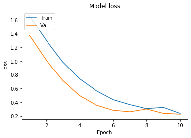

Confusion Matrix

• A confusion matrix is a table that is often used to describe the performance of a classification model (or "classifier") on a set of test data for which the true values are known.
• Each row of the matrix represents the instances in a predicted class while each column represents the instances in an actual class (or vice versa)
• The name stems from the fact that it makes it easy to see if the system is confusing two classes (i.e. commonly mislabeling one as another).
• All correct predictions are located in the diagonal of the table, so it is easy to visually inspect the table for prediction errors, as they will be represented by values outside the diagonal. For two classes the confusion matrix looks like this-

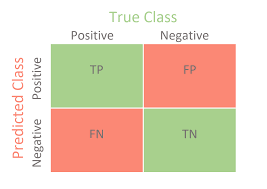
where:TP = True Positive; FP = False Positive; TN = True Negative; FN = False Negative.

Detailed video is available here: https://youtu.be/SToqP9V9y7Q

To calculate the confusion matrix we will use confusion_matrix from sklearn. We will be using mlxtend to plot the confusion matrix. You can install it using the command or from the link mentioned.

pip install mlxtend -> http://rasbt.github.io/mlxtend/installation/

from mlxtend.plotting import plot_confusion_matrix
from sklearn.metrics import confusion_matrix

predict_classes generates class predictions for the input samples.

y_pred = model.predict_classes(X_test)

mat = confusion_matrix(y_test, y_pred)
plot_confusion_matrix(conf_mat=mat, class_names=label.classes_, show_normed=True, figsize=(7,7))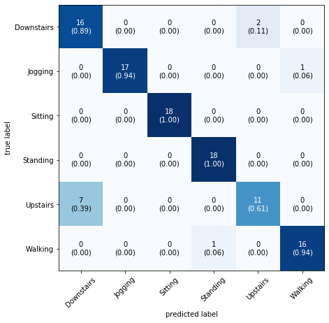

As you can see we are getting 100% accuracy for Sitting and Standing. The confusion matrix also tells us that our model is getting confused between Upstairs and Downstairs.

We have got a decent accuracy for this data. If you want to further increase the accuracy you can play around with many things. You can try traning the model with more data or you can even try tuning frame_size and hop_size.

Lastly, you can save the model using save_weights().

model.save_weights('model.h5')