How bagging works

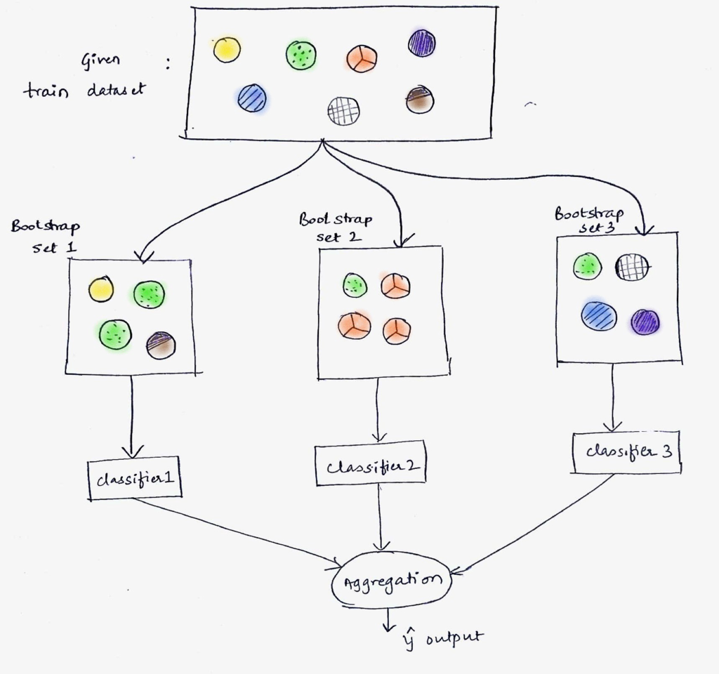
First of all we will try to understand what Bagging is from the following diagram:

Let’s say we have a dataset to train the model, first we need to divide this dataset into number of datasets(atleast more than 2).And then we need to apply `classifier on each of the dataset seperately then finally we do aggregationto get theoutput`.

SVM time complexity = O(n3)

i.e. As we increase number of input samples, training time increases cubically.

For Example

if 1000 input samples take 10 seconds to train then 3000 input samples might take 10 * 3^3 seconds to train.

If we divide 3000 samples into 3 categories each dataset contain 1000 samples. To train each dataset it will take 10sec in this way it will get over all time to train is 30sec(10+10+10). In this way we can improve training time of machine learning model.

Instead of 270sec, if we divide into 3 sets it will take 30sec.

Let’s have a look into the following script:

Importing required libraries

import numpy as np
from sklearn.ensemble import BaggingClassifier
from sklearn import datasets
from sklearn.svm import SVC

Importing iris dataset

iris = datasets.load_iris()
iris.keys()

dict_keys(['data', 'target', 'target_names', 'DESCR', 'feature_names', 'filename'])

Let’s see the description of the iris dataset

print(iris.DESCR)

.. _iris_dataset:

Iris plants dataset
--------------------

**Data Set Characteristics:**

    :Number of Instances: 150 (50 in each of three classes)
    :Number of Attributes: 4 numeric, predictive attributes and the class
    :Attribute Information:
        - sepal length in cm
        - sepal width in cm
        - petal length in cm
        - petal width in cm
        - class:
                - Iris-Setosa
                - Iris-Versicolour
                - Iris-Virginica
                
    :Summary Statistics:

    ============== ==== ==== ======= ===== ====================
                    Min  Max   Mean    SD   Class Correlation
    ============== ==== ==== ======= ===== ====================
    sepal length:   4.3  7.9   5.84   0.83    0.7826
    sepal width:    2.0  4.4   3.05   0.43   -0.4194
    petal length:   1.0  6.9   3.76   1.76    0.9490  (high!)
    petal width:    0.1  2.5   1.20   0.76    0.9565  (high!)
    ============== ==== ==== ======= ===== ====================

    :Missing Attribute Values: None
    :Class Distribution: 33.3% for each of 3 classes.
    :Creator: R.A. Fisher
    :Donor: Michael Marshall (MARSHALL%PLU@io.arc.nasa.gov)
    :Date: July, 1988

The famous Iris database, first used by Sir R.A. Fisher. The dataset is taken
from Fisher's paper. Note that it's the same as in R, but not as in the UCI
Machine Learning Repository, which has two wrong data points.

This is perhaps the best known database to be found in the
pattern recognition literature.  Fisher's paper is a classic in the field and
is referenced frequently to this day.  (See Duda & Hart, for example.)  The
data set contains 3 classes of 50 instances each, where each class refers to a
type of iris plant.  One class is linearly separable from the other 2; the
latter are NOT linearly separable from each other.

X = iris.data
y = iris.target

Let’s go ahead and get the shape of these x and y

X.shape, y.shape

((150, 4), (150,))

So x has 150 samples and 4 attributes . y has 150 samples.

We know 150 samples are less number of samples in machine leaning.So to get more number of samples we will use repeat() function .

We will repeat these 150 samples to 500 times then we will get 75000 samples.

X = np.repeat(X, repeats=500, axis = 0)
y = np.repeat(y, repeats=500, axis = 0)

X.shape, y.shape

((75000, 4), (75000,))

Train without Bagging

Now to train the model without bagging we will create a classifier called SVC() with linear kernel.

%%time
clf = SVC(kernel='linear', probability=True, class_weight='balanced')
clf.fit(X, y)
print('SVC: ', clf.score(X, y))

SVC:  0.98
Wall time: 34.5sec

Train it with Bagging

Now to train the model with bagging we will create a classifier called BaggingClassifier() with linear kernel.

%%time
n_estimators = 10
clf = BaggingClassifier(SVC(kernel='linear', probability=True, class_weight='balanced'), n_estimators=n_estimators, max_samples=1.0/n_estimators)
clf.fit(X, y)
print('SVC: ', clf.score(X, y))

SVC:  0.98
Wall time: 10.5 s

So from the above result we can observe improvement training time of the model from 34.5sec to 10.5sec.