K-Mean Clustering in Python | Machine Learning | KGP Talkie
What is K-Mean Clustering?
Machine Learning can broadly be classified into three types:
- Supervised Learning
- Unsupervised Learning
- Semi-supervised Learning
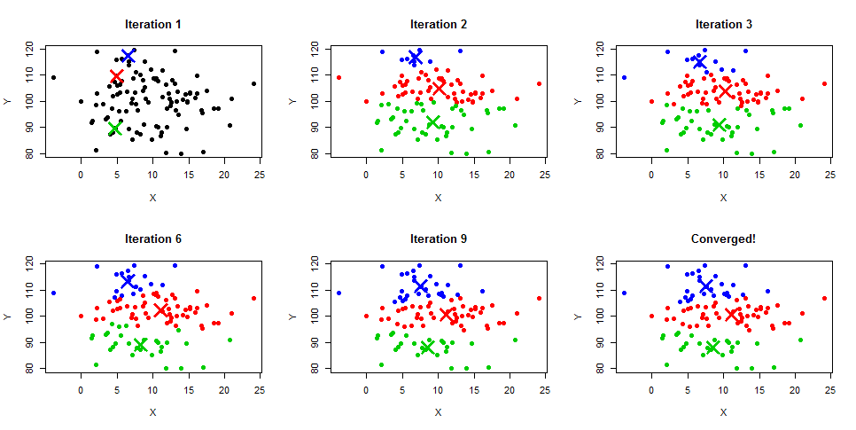
K-means algorithm identifies k number of centroids, and then allocates every data point to the nearest cluster, while keeping the centroids as small as possible. The ‘means’ in the K-means refers to averaging of the data; that is, finding the centroid.
Types of clustering
- Hard clustering
- Soft clustering
Type of Clustering Algorithms
Connectivity-based clustering
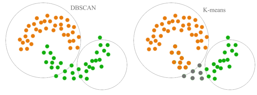
The main idea behind this clustering is that data points that are closer in the data space are more related (similar) than to data points farther away. They are also not very robust towards outliers, which might show up as additional clusters or even cause other clusters to merge.
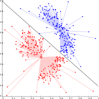
Centroid-based clustering
In this type of clustering, clusters are represented by a central vector or a centroid. This centroid might not necessarily be a member of the dataset.
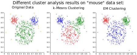
Distribution-based clustering
These models have a strong theoritical foundation, however they often suffer from overfitting. Gaussian mixture models, using the expectation-maximization algorithm is a famous distribution based clustering method.
Density-based methods search the data space for areas of varied density of data points.
Dataset and Problem Understanding
At first we will be importing certain libraries which we will need to work on the given dataset.
Pandas which offers data structures and operation for manipulating numerical tables.
Seaborn and matplotlib for data visualizations.
Also numpy for working on array.
import pandas as pd
import numpy as np
import seaborn as sns
import matplotlib.pyplot as plt
%matplotlib inline
Fetching the data using pandas.
data = pd.read_csv('data.csv', index_col = 0)
data.head()| x | y | cluster | |
|---|---|---|---|
| 0 | -8.482852 | -5.603349 | 2 |
| 1 | -7.751632 | -8.405334 | 2 |
| 2 | -10.967098 | -9.032782 | 2 |
| 3 | -11.999447 | -7.606734 | 2 |
| 4 | -1.736810 | 10.478015 | 1 |
Let’s look at the top five rows using the Dataframe’s head() method. you can find out what all categories exist and how many instances(row) belong to each category by using value_counts() method .
data['cluster'].value_counts()
1    67
0    67
2    66
Name: cluster, dtype: int64
So, we have 67 dataset each which belong to cluster 1 and cluster 0 and 66 dataset belong to cluster 2.
Now we can a scatter plot of the dataset and visualize the cluster formed.
We have matplotlib library which we have already impoted above to plot the dataset. So before you can plot anything, you need to specify which backend Matplotlib should use. The simplest option is to use Jupyter’s magic command %matplotlib inline. This tells Jupyter to set up Matplotlib so it uses Jupyter’s own backend.
plt.scatter(data['x'], data['y'], c = data['cluster'], cmap = 'viridis')
plt.xlabel('X-values')
plt.ylabel('Y-values')
plt.title('Formation of cluster')
plt.show()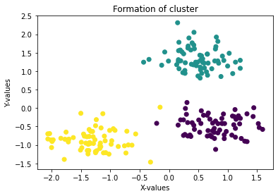
K-Means for clustering
The K-Means algorithm is a simple algorithm capable of clustering the same kind of dataset very quickly and efficiently, often in just a few iterations.Its an unsupervised machine learning technique.
Let’s train a K-Means cluster on this dataset. It will try to find each blob's center and assign each instance to the closed blob.
Importing K – Means from sklearn cluster at first.
from sklearn.cluster import KMeans
from sklearn.preprocessing import StandardScaler
X = data[['x', 'y']]
y = data['cluster']
We standardize the dataset before training the algorithm because the variable can of incomparable units (eg one in cm other in kg) so we should standardize variables, ofcourse. Also when the data show quite a different variances it is a good practice to standardize the data
scaler = StandardScaler()
X = scaler.fit_transform(X)
X[: 5]
array([[-1.01200363, -0.60606415],
       [-0.86550679, -1.04265203],
       [-1.5097118 , -1.14041707],
       [-1.71653856, -0.91821912],
       [ 0.33953731,  1.89963378]])
Now we impute back the standardized data in our dataset and train the algorithm.
data[['x', 'y']] = X
We are taking the number of clusters k as two for time being.
Note that you have to specify the number of clusters k that the algorithm must find. In this dataset, it is pretty obvious from looking at the data that k should be set to 3, but we choose it 2 as of now. Also in general it is not that easy to find the number of clusters.
Later we will see the method to find the optimal number of cluster for a dataset.
k=2
kmeans = KMeans(n_clusters=k, random_state=42)
kmeans.fit(X)
KMeans(n_clusters=2, random_state=42)
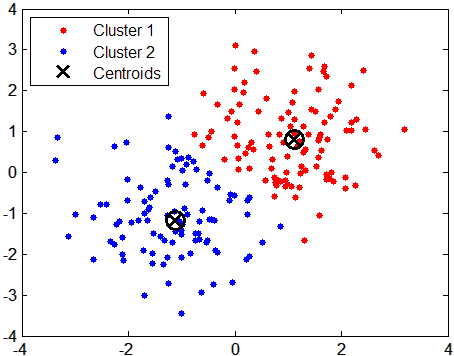
We will take a look at the two centroid that the algorithm found:
center = kmeans.cluster_centers_
center
array([[-1.30618271, -0.87560626],
       [ 0.64334372,  0.43126875]])
Now plotting the dataset and each centroid.
plt.scatter(data['x'], data['y'], c = kmeans.labels_, cmap = 'viridis')
plt.xlabel('X-values')
plt.ylabel('Y-values')
plt.title('Formation of cluster with centroids')
for i, point in enumerate(center):
    plt.plot(center[i][0], center[i][1], '*r--', linewidth=2, markersize=18)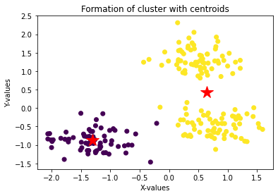
With number of cluster as 2 thecentroid (marked as red star above) are pretty obivious.
plt.scatter(data['x'], data['y'], c = data['cluster'], cmap = 'viridis')
plt.xlabel('X-values')
plt.ylabel('Y-values')
plt.title('Formation of 3-cluster')
plt.show()
here we can easily visualize 3 clusters. So, now we will see how we can find out the right value for K (number of cluster)
How do I choose right value of k?
you need to understand how it works?
Assuming we have inputs x_1, x_2, x_3, …, x_nx
- Step 1 – Pick K random points as cluster centers called centroids.
- Step 2 – Assign each x_i to nearest cluster by calculating its distance to each centroid.
- Step 3 – Find new cluster center by taking the average of the assigned points.
- Step 4 – Repeat Step 2 and 3 until none of the cluster assignments change.

Most important, when to stop increasing K?
We often know the value of K. In that case we use the value of K. Else we use the Elbow Method.
Error Sum of Squares (SSE)
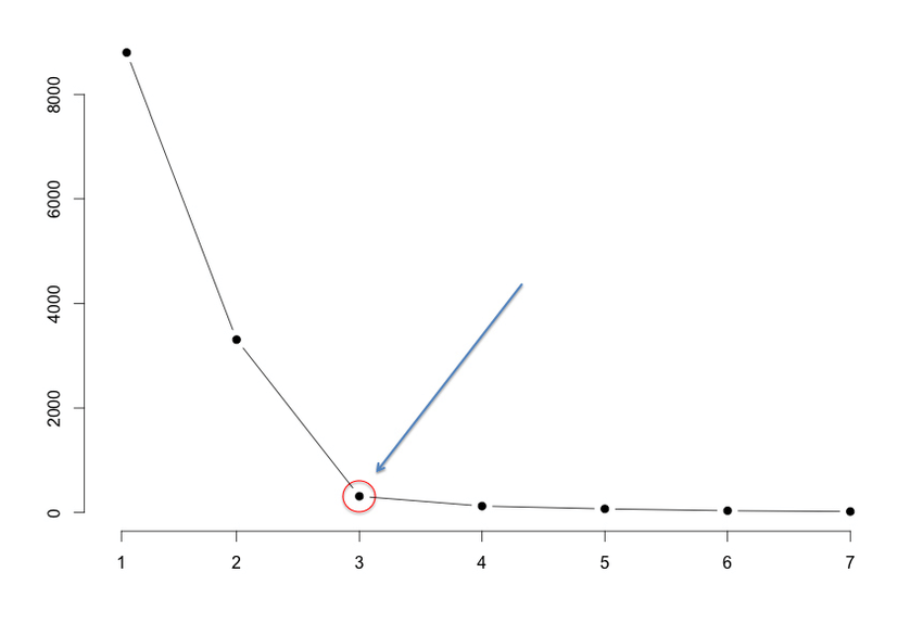
It is the sum of the squared differences between each observation and its group’s mean. We can use it as a measure of variation within a cluster. All cases within a cluster are identical then SSE would be equal to 0. We run the algorithm for different values of K(say K = 10 to 1) and plot the K values against SSE(Sum of Squared Errors). And select the value of K for the elbow point as shown in the figure.
$$ \text SSE = \sum_{i=1}^k\left(\sum_{x_j \subset S_i}||x_j-\mu_i||^2\right) $$
So we try value for k between 1 to 10 and use elbow method as explaind above.
SSE = []
index = range(1,10)
for i in index:
    kmeans = KMeans(n_clusters=i, random_state=42)
    kmeans.fit(X)
    SSE.append(kmeans.inertia_)
    print(kmeans.inertia_)
400.0000000000001 156.41078579574975 44.057048453292815 36.726387118666075 31.01642761531463 25.39959047192452 22.547184727743304 19.92343817847746 17.295836404824982
Here the metric inertia is nothing but the mean squared distance between each instance and its closest centroid.
plt.plot(index, SSE)
plt.xlabel('K')
plt.ylabel('SEE')
plt.title('SSE with respect to K')
plt.show()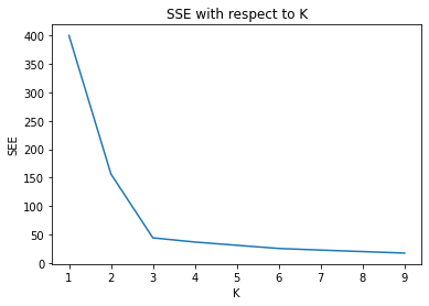
From the graph, we can observe with increasing the K value SSE will decrease. So, like mentioned before the value of k should be 3. Now lets do it again with k=3
k=3
kmeans = KMeans(n_clusters=k, random_state=42)
kmeans.fit(X)
KMeans(n_clusters=3, random_state=42)
center = kmeans.cluster_centers_
plt.xlabel('X-values')
plt.ylabel('Y-values')
plt.title('Formation of clusters with 3-centroids')

plt.scatter(data['x'], data['y'], c = kmeans.labels_, cmap = 'viridis')
for i, point in enumerate(center):
plt.plot(center[i][0], center[i][1], '*r--', linewidth=2, markersize=18)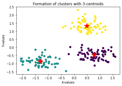
Let’s go ahead and explore it in a little bit more detail
Use Iris dataset
from sklearn import datasets
iris = datasets.load_iris()
X = iris.data
scaler = StandardScaler()
X = scaler.fit_transform(X)
iris.target_names
array(['setosa', 'versicolor', 'virginica'], dtype='<U10')
SSE = []
index = range(1,10)
for i in index:
    kmeans = KMeans(n_clusters=i, random_state=42)
    kmeans.fit(X)
    SSE.append(kmeans.inertia_)
    print(kmeans.inertia_)
600.0 222.36170496502302 139.82049635974974 114.41256181896094 90.92751382392049 80.0224959955744 71.81624598106144 62.28749580350205 54.8110520315013
plt.plot(index, SSE)
plt.xlabel('K')
plt.ylabel('SSE')
plt.title('Variation of SSE with respect to K')
plt.show()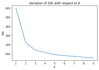
0 Comments