What is Regularisation?

Regularization adds a penalty on the different parameters of the model to reduce the freedom of the model. Hence, the model will be less likely to fit the noise of the training data and will improve the generalization abilities of the model.

There are basically 3-types of regularization

• L1 regularization (also called Lasso) It shrinks the co-efficients which are less important to zero. That means with Lasso regularization we can remove some features.
• L2 regularization (also called Ridge) It does't reduce the co-efficients to zero`` but it reduces the regression co-efficients with this reduction we can identify which feature has more important.
• L1/L2 regularization (also called Elastic net)

What is Lasso Regularisation

3 sources of error

• Noise We can't do anything with the noise. Let's focus on following errors.
• Bias error
  It is useful to quantify how much on an average are the predicted values different from the actual value.
• Variance
  On the other side quantifies how are the prediction made on the same observation different from each other.

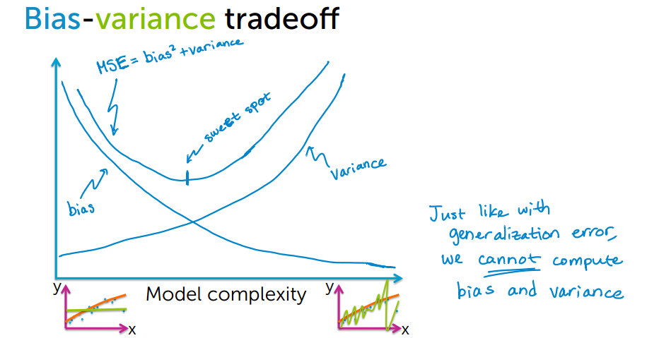
Now we will try to understand bias - variance trade off from the following figure.
By increasing model complexity, total error will decrease till some point and then it will start to increase. W need to select optimum model complexity to get less error.

For low complexity model : high bias and low variance
For high complexity model : low bias and high variance

If you are getting high bias then you have a fair chance to increase model complexity. And otherside it you are getting high variance, you need to decrease model complexity that's how any machine learning algorithm works.

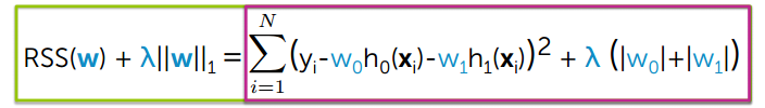
w is the regression co-efficient
λ is the regularization co-efficient.

The L1 regularization adds a penalty equal to the sum of the absolute value of the coefficients.

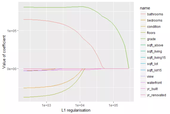
We can observe from the following figure. The L1 regularization will shrink some parameters to zero. Hence some variables will not play any role in the model to get final output, L1 regression can be seen as a way to select features in a model.

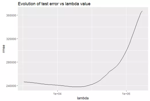
Let's observe the evolution of test error by changing the value of λ

from the following figure.

How to choose λ

Let's move ahead and choose the best λ.

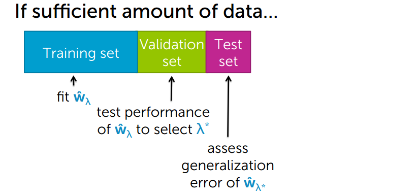
We have a sufficient amount of data. In that we can split our data into 3 sets those are

• Training set
• Validation set
• Test set

• In the training set, we fit our model and set regression co-efficients with the regularization.
• Then we test our model's performance to select λ

• on validation set, if any thing wrong with the model like less accuracy we validate on the validation set then we change the parameter the we go back to the training set and do the optimization.
• Finally, it will do generalize testing on the test set.

What is Ridge Regularisation?

Let's first understand what exactly Ridge regularization:

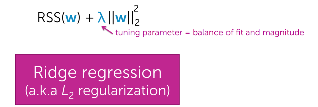
The L2 regularization adds a penalty equal to the sum of the squared value of the coefficients.

λ is the tuning parameter or optimization parameter.
w is the regression co-efficient.

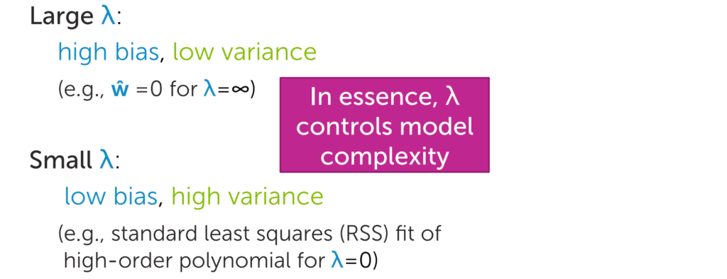
In this regularization,
if λ is high then we will get high bias and low variance.
if λ is low then we will get low bias and high variance.

So what we do we will find out the optimized value of λ by tuning the parameters. And we can say λ is the strength of the regularization.

The L2 regularization will force the parameters to be relatively small, the bigger the penalization, the smaller (and the more robust) the coefficients are.

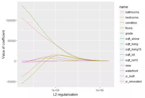
When we compare this plot to the L1 regularization plot, we notice that the coefficients decrease progressively and are not cut to zero. They slowly decrease to zero.

Load the titanic data

Importing required libraries:

import numpy as np
import pandas as pd
import seaborn as sns
import matplotlib.pyplot as plt
%matplotlib inline

from sklearn.model_selection import train_test_split
from sklearn.ensemble import RandomForestClassifier
from sklearn.linear_model import Lasso, LogisticRegression
from sklearn.feature_selection import SelectFromModel
from sklearn.preprocessing import StandardScaler
from sklearn.metrics import accuracy_score

titanic = sns.load_dataset('titanic')
titanic.isnull().sum()

survived         0
pclass           0
sex              0
age            177
sibsp            0
parch            0
fare             0
embarked         2
class            0
who              0
adult_male       0
deck           688
embark_town      2
alive            0
alone            0
dtype: int64

Remove age and deck features from the titanice data

titanic.drop(labels = ['age', 'deck'], axis = 1, inplace = True)

titanic = titanic.dropna()
titanic.isnull().sum()

survived       0
pclass         0
sex            0
sibsp          0
parch          0
fare           0
embarked       0
class          0
who            0
adult_male     0
embark_town    0
alive          0
alone          0
dtype: int64

titanic.head()

	survived	pclass	sex	sibsp	parch	fare	embarked	class	who	adult_male	embark_town	alive	alone
0	0	3	male	1	0	7.2500	S	Third	man	True	Southampton	no	False
1	1	1	female	1	0	71.2833	C	First	woman	False	Cherbourg	yes	False
2	1	3	female	0	0	7.9250	S	Third	woman	False	Southampton	yes	True
3	1	1	female	1	0	53.1000	S	First	woman	False	Southampton	yes	False
4	0	3	male	0	0	8.0500	S	Third	man	True	Southampton	no	True

data = titanic[['pclass', 'sex', 'sibsp', 'parch', 'embarked', 'who', 'alone']].copy()

data.head()

	pclass	sex	sibsp	parch	embarked	who	alone
0	3	male	1	0	S	man	False
1	1	female	1	0	C	woman	False
2	3	female	0	0	S	woman	True
3	1	female	1	0	S	woman	False
4	3	male	0	0	S	man	True

sex = {'male': 0, 'female': 1}
data['sex'] = data['sex'].map(sex)                       ports = {'S': 0, 'C': 1, 'Q': 2}
data['embarked'] = data['embarked'].map(ports)             who = {'man': 0, 'woman': 1, 'child': 2}
data['who'] = data['who'].map(who)                       alone = {True: 1, False: 0}
data['alone'] = data['alone'].map(alone)

Load the data into x

X = data.copy()
y = titanic['survived']
x.head()

No.	pclass	sex	sibsp	parch	embarked	who	alone
0	3	0	1	0	0	0	0
1	1	1	1	0	1	1	0
2	3	1	0	0	0	1	1
3	1	1	1	0	0	1	0
4	3	0	0	0	0	0	1

X_train, X_test, y_train, y_test = train_test_split(X, y, test_size = 0.33, random_state = 42)

SelectFromModel( )

It is a meta-transformer for selecting features based on importance weights.

sel = SelectFromModel(LogisticRegression(C = 0.05, penalty = 'l1', solver = 'liblinear'))
sel.fit(X_train, y_train)

SelectFromModel(estimator=LogisticRegression(C=0.05, penalty='l1', solver='liblinear'))                                     

get_support( )

By using this, we will get a mask or integer index, of the features selected.

sel.get_support()

array([ True,  True,  True, False, False,  True, False])

features = X_train.columns[sel.get_support()]
features

Index(['pclass', 'sex', 'sibsp', 'who'], dtype='object')

Let's get the transformed version of x_train and x_test

X_train_l1 = sel.transform(X_train)
X_test_l1 = sel.transform(X_test)
X_train_l1.shape, X_test_l1.shape

((595, 4), (294, 4))

Build ML model and compare performance

Let's implement the randomForest function and we wil do the training of the model.

def run_randomForest(X_train, X_test, y_train, y_test):
    clf = RandomForestClassifier(n_estimators=100, random_state=0, n_jobs = -1)
    clf.fit(X_train, y_train)
    y_pred = clf.predict(X_test)
    print('Accuracy: ', accuracy_score(y_test, y_pred))

Let's get the accuracy between test and trained data and wall time by using run_randomForest( )

%%time
run_randomForest(X_train_l1, X_test_l1, y_train, y_test)

Accuracy:  0.826530612244898
Wall time: 517 ms

%%time
run_randomForest(X_train, X_test, y_train, y_test)

Accuracy:  0.8163265306122449
Wall time: 169 ms

Ridge Regression

from sklearn.linear_model import RidgeClassifier

rr = RidgeClassifier(alpha=300)
rr.fit(X_train, y_train)               RidgeClassifier(alpha=300)

Let's get the accuracy between x_test and y_test by using the function score()

rr.score(X_test, y_test)

0.8231292517006803

Let's get the co-efficients of the regression

rr.coef_

array([[-0.20537487,  0.24017869, -0.07964489, -0.00072071,  0.05154718, 0.26474716, -0.07454003]])

from sklearn.linear_model import RidgeClassifierCV

RidgeClassifierCV( )

It performs Generalized Cross-Validation, which is a form of efficient Leave-One-Out cross-validation.

rr = RidgeClassifierCV(alphas=[10, 20, 50, 100, 200, 300], cv = 10 )
rr.fit(X_train, y_train)        RidgeClassifierCV(alphas=array([ 10, 20, 50, 100, 200, 300]), cv=10)

Now will get the accuracy between x_test and y_test by using score()

rr.score(X_test, y_test)

0.8197278911564626

rr.coef_

array([[-0.23422431,  0.29215915, -0.09681069, -0.01263653,  0.05860246, 0.31323408, -0.09073738]])
   

rr.alpha_

200

rr.alphas

array([ 10,  20,  50, 100, 200, 300])