What is it?

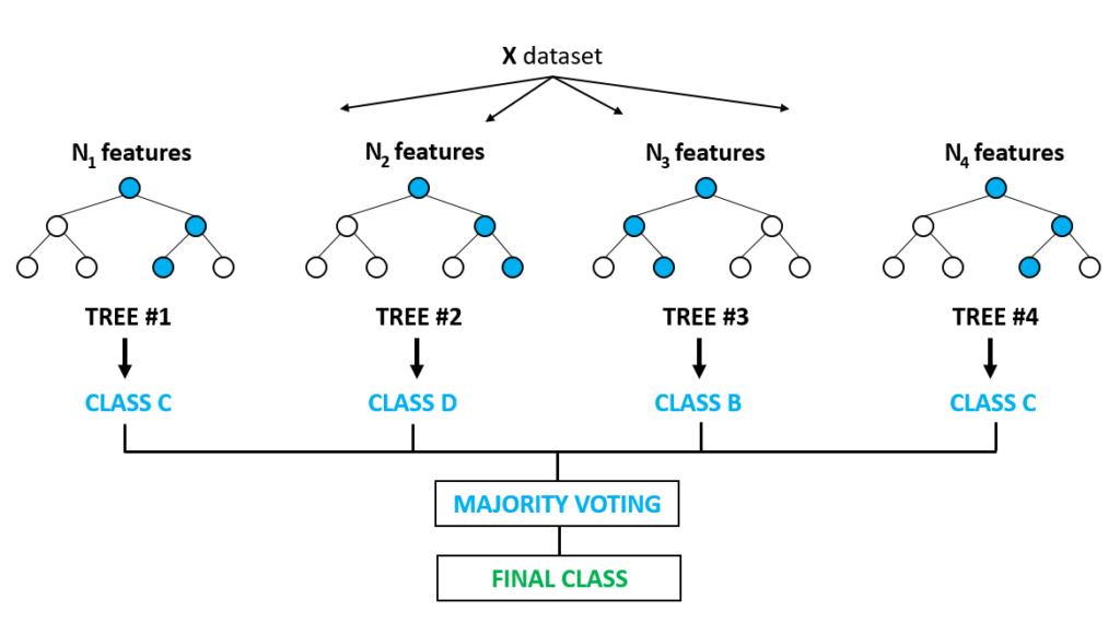
A Random Forest is an ensemble technique which can have capable of performing both regression and classification tasks with the use of multiple decision trees and a technique called Bootstrap and Aggregation, commonly known as bagging. The basic idea behind this is to combine multiple decision trees in determining the final output rather than relying on individual decision trees. Random forests has a variety of applications, such as recommendation engines, image classification and feature selection. It can be used to classify loyal loan applicants, identify fraudulent activity and predict diseases. It lies at the base of the Boruta algorithm, which selects important features in a dataset.

How the Random Forest Algorithm Works

• Select random samples from a given dataset.
• Construct a decision tree for each sample and get a prediction result from each decision tree.
• Perform a vote for each predicted result.
• Select the prediction result with the most votes as the final prediction.

Important Feature for Classification

Random forest uses gini importance ormean decrease in impurity (MDI) to calculate the importance of each feature. Gini importance is also known as the total decrease in node impurity. This is how much the model fit or accuracy decreases when you drop a variable. The larger the decrease, the more significant the variable is. Here, the mean decrease is a significant parameter for variable selection. The Gini index can describe the overall explanatory power of the variables.

Random Forests vs Decision Trees

• Random forests is a set of multiple decision trees.
• Deep decision trees may suffer from overfitting, but random forests prevents overfitting by creating trees on random subsets.
• Decision trees are computationally faster.
• Random forests is difficult to interpret, while a decision tree is easily interpretable and can be converted to rules.

Part 1: Random Forest as a Regression

import pandas as pd
import numpy as np
import seaborn as sns
import matplotlib.pyplot as plt
%matplotlib inline

from sklearn import datasets, metrics
from sklearn.model_selection import train_test_split
from sklearn.ensemble import RandomForestRegressor

diabetes = datasets.load_diabetes()
diabetes.keys()

dict_keys(['data', 'target', 'frame', 'DESCR', 'feature_names', 'data_filename', 'target_filename'])

print(diabetes.DESCR)

.. _diabetes_dataset:

Diabetes dataset
----------------

Ten baseline variables, age, sex, body mass index, average blood
pressure, and six blood serum measurements were obtained for each of n =
442 diabetes patients, as well as the response of interest, a
quantitative measure of disease progression one year after baseline.

**Data Set Characteristics:**

  :Number of Instances: 442

  :Number of Attributes: First 10 columns are numeric predictive values

  :Target: Column 11 is a quantitative measure of disease progression one year after baseline

  :Attribute Information:
      - age     age in years
      - sex
      - bmi     body mass index
      - bp      average blood pressure
      - s1      tc, T-Cells (a type of white blood cells)
      - s2      ldl, low-density lipoproteins
      - s3      hdl, high-density lipoproteins
      - s4      tch, thyroid stimulating hormone
      - s5      ltg, lamotrigine
      - s6      glu, blood sugar level

Note: Each of these 10 feature variables have been mean centered and scaled by the standard deviation times `n_samples` (i.e. the sum of squares of each column totals 1).

we will see the dimensions of X & Y:

X = diabetes.data
y = diabetes.target
X.shape, y.shape

((442, 10), (442,))

X_train, X_test, y_train, y_test = train_test_split(X, y, test_size = 0.3, random_state = 42)

RandomForestRegressor()

A random forest is a meta estimator that fits a number of classifying decision trees on various sub-samples of the dataset and uses averaging to improve the predictive accuracy and control over-fitting.Let's look at script:

regressor = RandomForestRegressor(n_estimators=100, random_state = 42)
regressor.fit(X_train, y_train)
y_pred = regressor.predict(X_test)

The following plot shows predicted data of y and testing data of y.

plt.figure(figsize=(16,4))
plt.plot(y_pred,  label='y_pred')
plt.plot(y_test, label='y_test')
plt.xlabel('X_test', fontsize=14)
plt.ylabel('Value of y(pred , test)', fontsize=14)
plt.title('Comparing predicted values and true values')
plt.legend(title='Parameter where:')
plt.show()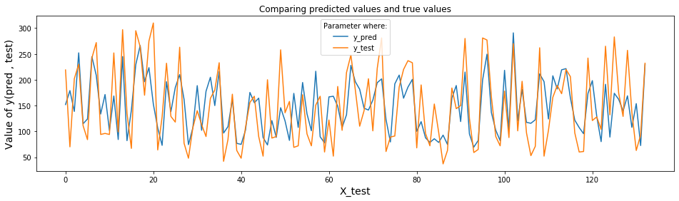

Let's see the Root Mean Square Error of data.To get this we will use function called mean_squared_error().Now, have a look at following code:

np.sqrt(metrics.mean_squared_error(y_test, y_pred))

53.505825893179875

(72.78-53.50)/72.78

0.26490794174223686

y_test.std()

73.47317715932746

Random Forest as a Classifier with iris dataset

from sklearn.ensemble import RandomForestClassifier

iris = datasets.load_iris()     
iris.target_names                             

array(['setosa', 'versicolor', 'virginica'], dtype='<U10')

print(iris.DESCR)

.. _iris_dataset:

Iris plants dataset
--------------------

**Data Set Characteristics:**

    :Number of Instances: 150 (50 in each of three classes)
    :Number of Attributes: 4 numeric, predictive attributes and the class
    :Attribute Information:
        - sepal length in cm
        - sepal width in cm
        - petal length in cm
        - petal width in cm
        - class:
                - Iris-Setosa
                - Iris-Versicolour
                - Iris-Virginica
                
    :Summary Statistics:

    ============== ==== ==== ======= ===== ====================
                    Min  Max   Mean    SD   Class Correlation
    ============== ==== ==== ======= ===== ====================
    sepal length:   4.3  7.9   5.84   0.83    0.7826
    sepal width:    2.0  4.4   3.05   0.43   -0.4194
    petal length:   1.0  6.9   3.76   1.76    0.9490  (high!)
    petal width:    0.1  2.5   1.20   0.76    0.9565  (high!)
    ============== ==== ==== ======= ===== ====================

    :Missing Attribute Values: None
    :Class Distribution: 33.3% for each of 3 classes.
    :Creator: R.A. Fisher
    :Donor: Michael Marshall (MARSHALL%PLU@io.arc.nasa.gov)
    :Date: July, 1988

The famous Iris database, first used by Sir R.A. Fisher. The dataset is taken
from Fisher's paper. Note that it's the same as in R, but not as in the UCI
Machine Learning Repository, which has two wrong data points.

This is perhaps the best known database to be found in the
pattern recognition literature.  Fisher's paper is a classic in the field and
is referenced frequently to this day.  (See Duda & Hart, for example.)  The
data set contains 3 classes of 50 instances each, where each class refers to a
type of iris plant.  One class is linearly separable from the other 2; the
latter are NOT linearly separable from each other.

Use iris data set:

X = iris.data
y = iris.target

X_train, X_test, y_train, y_test = train_test_split(X, y, random_state = 1, test_size = 0.3, stratify = y)

clf = RandomForestClassifier(n_estimators=100, random_state = 42)
clf.fit(X_train, y_train)          RandomForestClassifier(random_state=42)

predict()

In a given trained model, predict the label of a new set of data. This method accepts one argument, the new data X_test , and returns the learned label for each object in the array.

y_pred = clf.predict(X_test)
print(metrics.accuracy_score(y_test, y_pred))

0.9777777777777777

mat = metrics.confusion_matrix(y_test, y_pred)
mat

array([[15,  0,  0],
       [ 0, 15,  0],
       [ 0,  1, 14]], dtype=int64)

Confusion_matrix ( )

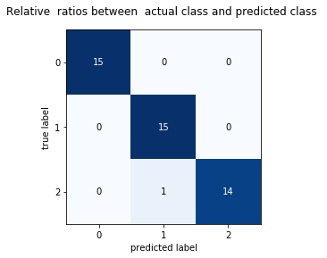
The diagonal elements represent the number of points for which the predicted label is equal to the true label, while off-diagonal elements are those that are mislabeled by the classifier. The higher the diagonal values of the confusion matrix the better, indicating many correct predictions.
Each cell in the square box represents relateve or absolute ratios between y_test and y_pred .

Let's try to plot output of classifier by using confusion_matrix () function to represent with respected colors.Now look into the following script:

from mlxtend.evaluate import confusion_matrix
from mlxtend.plotting import plot_confusion_matrix
print('Confusion Matrix')
cm = confusion_matrix(y_test, y_pred)
fig, ax = plot_confusion_matrix(conf_mat = cm  )
plt.title('Relative  ratios between  actual class and predicted class ')
plt.show()

Confusion Matrix

clf.feature_importances_ 

array([0.1160593 , 0.03098375, 0.43034957, 0.42260737])

iris.feature_names

['sepal length (cm)',
 'sepal width (cm)',
 'petal length (cm)',
 'petal width (cm)']