What is Support Vector Machines (SVM)

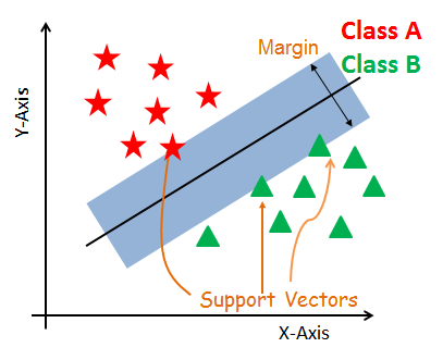
We will start our discussion with little introduction about SVM. Support Vector Machine(SVM) is a supervised binary classification algorithm. Given a set of points of two types in N-dimensional place SVM generates a (N−1) dimensional hyperplane to separate those points into two groups.

A SVM classifier would attempt to draw a straight line separating the two sets of data, and thereby create a model for classification. For two dimensional data like that shown here, this is a task we could do by hand. But immediately we see a problem: there is more than one possible dividing line that can perfectly discriminate between the two classes.

• Support Vectors
• Hyperplane
• Margin

Support Vectors

Support vectors are the data points, which are closest to the hyperplane. These points will define the separating line better by calculating margins. These points are more relevant to the construction of the classifier.

Hyperplane

A hyperplane is a decision plane which separates between a set of objects having different class memberships.

Margin

A margin is a gap between the two lines on the closest class points. This is calculated as the perpendicular distance from the line to support vectors or closest points. If the margin is larger in between the classes, then it is considered a good margin, a smaller margin is a bad margin.

How SVM works?

• Generate hyperplanes which segregates the classes in the best way. Left-hand side figure showing three hyperplanes black, blue and orange. Here, the blue and orange have higher classification error, but the black is separating the two classes correctly.

• Select the right hyperplane with the maximum segregation from the either nearest data points as shown in the right-hand side figure.

Separation Planes

• Linear
• Non-Linear

Dealing with non-linear and inseparable planes

SVM uses a kernel trick to transform the input space to a higher dimensional space

Beauty of Kernal

kernels allow us to do stuff in infinite dimensions. Sometimes going to higher dimension is not just computationally expensive, but also impossible. function can be a mapping from n-dimension to infinite dimension which we may have little idea of how to deal with. Then kernel gives us a wonderful shortcut.

SVM Kernels

• Linear
• Polynomial
• Radial Basis Function

The SVM algorithm is implemented in practice using a kernel. Kernel helps you to build a more accurate classifier.

• A linear kernel can be used as normal dot product any two given observations. The product between two vectors is the sum of the multiplication of each pair of input values.Training a SVM with a Linear Kernel is Faster than with any other Kernel.
• A polynomial kernel is a more generalized form of the linear kernel. The polynomial kernel can distinguish curved or nonlinear input space.
• The Radial basis function (RBF) kernel is a popular kernel function commonly used in Support Vector Machine classification. RBF can map an input space in infinite dimensional space.

Let's Build Model in sklearn

import pandas as pd
import seaborn as sns
import matplotlib.pyplot as plt
import numpy as np

from sklearn import datasets, metrics
from sklearn.model_selection import train_test_split
from sklearn.preprocessing import StandardScaler

cancer = datasets.load_breast_cancer()
cancer.keys()
dict_keys(['data', 'target', 'frame', 'target_names', 'DESCR', 'feature_names', 'filename'])
print(cancer.DESCR)

.. _breast_cancer_dataset:

Breast cancer wisconsin (diagnostic) dataset
--------------------------------------------

**Data Set Characteristics:**

    :Number of Instances: 569

    :Number of Attributes: 30 numeric, predictive attributes and the class

    :Attribute Information:
        - radius (mean of distances from center to points on the perimeter)
        - texture (standard deviation of gray-scale values)
        - perimeter
        - area
        - smoothness (local variation in radius lengths)
        - compactness (perimeter^2 / area - 1.0)
        - concavity (severity of concave portions of the contour)
        - concave points (number of concave portions of the contour)
        - symmetry
        - fractal dimension ("coastline approximation" - 1)

        The mean, standard error, and "worst" or largest (mean of the three
        worst/largest values) of these features were computed for each image,
        resulting in 30 features.  For instance, field 0 is Mean Radius, field
        10 is Radius SE, field 20 is Worst Radius.

        - class:
                - WDBC-Malignant
                - WDBC-Benign

    :Summary Statistics:

    ===================================== ====== ======
                                           Min    Max
    ===================================== ====== ======
    radius (mean):                        6.981  28.11
    texture (mean):                       9.71   39.28
    perimeter (mean):                     43.79  188.5
    area (mean):                          143.5  2501.0
    smoothness (mean):                    0.053  0.163
    compactness (mean):                   0.019  0.345
    concavity (mean):                     0.0    0.427
    concave points (mean):                0.0    0.201
    symmetry (mean):                      0.106  0.304
    fractal dimension (mean):             0.05   0.097
    radius (standard error):              0.112  2.873
    texture (standard error):             0.36   4.885
    perimeter (standard error):           0.757  21.98
    area (standard error):                6.802  542.2
    smoothness (standard error):          0.002  0.031
    compactness (standard error):         0.002  0.135
    concavity (standard error):           0.0    0.396
    concave points (standard error):      0.0    0.053
    symmetry (standard error):            0.008  0.079
    fractal dimension (standard error):   0.001  0.03
    radius (worst):                       7.93   36.04
    texture (worst):                      12.02  49.54
    perimeter (worst):                    50.41  251.2
    area (worst):                         185.2  4254.0
    smoothness (worst):                   0.071  0.223
    compactness (worst):                  0.027  1.058
    concavity (worst):                    0.0    1.252
    concave points (worst):               0.0    0.291
    symmetry (worst):                     0.156  0.664
    fractal dimension (worst):            0.055  0.208
    ===================================== ====== ======

    :Missing Attribute Values: None

    :Class Distribution: 212 - Malignant, 357 - Benign

    

cancer.target_names
array(['malignant', 'benign'], dtype='<U9')
cancer.feature_names[: 5]

array(['mean radius', 'mean texture', 'mean perimeter', 'mean area',
       'mean smoothness'], dtype='<U23')

cancer.feature_names.shape

(30,)

X = cancer.data
y = cancer.target
X.shape, y.shape

((569, 30), (569,))

Let's print the slicing array of x , y:

X[: 2]

array([[1.799e+01, 1.038e+01, 1.228e+02, 1.001e+03, 1.184e-01, 2.776e-01,
        3.001e-01, 1.471e-01, 2.419e-01, 7.871e-02, 1.095e+00, 9.053e-01,
        8.589e+00, 1.534e+02, 6.399e-03, 4.904e-02, 5.373e-02, 1.587e-02,
        3.003e-02, 6.193e-03, 2.538e+01, 1.733e+01, 1.846e+02, 2.019e+03,
        1.622e-01, 6.656e-01, 7.119e-01, 2.654e-01, 4.601e-01, 1.189e-01],
       [2.057e+01, 1.777e+01, 1.329e+02, 1.326e+03, 8.474e-02, 7.864e-02,
        8.690e-02, 7.017e-02, 1.812e-01, 5.667e-02, 5.435e-01, 7.339e-01,
        3.398e+00, 7.408e+01, 5.225e-03, 1.308e-02, 1.860e-02, 1.340e-02,
        1.389e-02, 3.532e-03, 2.499e+01, 2.341e+01, 1.588e+02, 1.956e+03,
        1.238e-01, 1.866e-01, 2.416e-01, 1.860e-01, 2.750e-01, 8.902e-02]])

y[: 10]

array([0, 0, 0, 0, 0, 0, 0, 0, 0, 0])

Standardization

Standardization of a dataset is a common requirement for many machine learning estimators: they might behave badly if the individual feature do not more or less look like standard normally distributed data (e.g. Gaussian with 0 mean and unit variance).
The idea behind StandardScaler() is that it will transform your data such that its distribution will have a mean value 0 and standard deviation of 1.

scaler = StandardScaler()
X_scaled = scaler.fit_transform(X)
X_scaled[2:2]

array([], shape=(0, 30), dtype=float64)

Split the data and build the model

X_train, X_test, y_train, y_test = train_test_split(X_scaled, y, test_size = 0.2, random_state = 1, stratify = y)

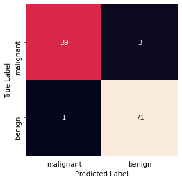
Linear kernel

Let’s create a Linear Kernel SVM using the sklearn library of Python. Linear Kernel is used when the data is Linearly separable, that is, it can be separated using a single Line. It is one of the most common kernels to be used. It is mostly used when there are a Large number of Features in a particular Data Set.

from sklearn import svm

clf = svm.SVC(kernel='linear')
clf.fit(X_train, y_train)
y_predict = clf.predict(X_test)

print('Accuracy: ', metrics.accuracy_score(y_test, y_predict))

print('Precision: ', metrics.precision_score(y_test, y_predict))
print('Recall: ', metrics.recall_score(y_test, y_predict))

print('Confusion Matrix')

mat = metrics.confusion_matrix(y_test, y_predict)
sns.heatmap(mat, square = True, annot = True, fmt = 'd', cbar = False,
           xticklabels=cancer.target_names,
           yticklabels=cancer.target_names)

plt.xlabel('Predicted Label')
plt.ylabel('True Label')
plt.show()

Accuracy:  0.9649122807017544
Precision:  0.9594594594594594
Recall:  0.9861111111111112
Confusion Matrix

np.unique()

This function returns an array of unique elements in the input array. The function can be able to return a tuple of array of unique vales and an array of associated indices. Nature of the indices depend upon the type of return parameter in the function call.
Let's see the following code:

element, count = np.unique(y_test, return_counts=True)
element, count

(array([0, 1]), array([42, 72], dtype=int64))

X_train, X_test, y_train, y_test = train_test_split(X, y, test_size = 0.2, random_state = 1, stratify = y)

clf = svm.SVC(kernel='linear')
clf.fit(X_train, y_train)
y_predict = clf.predict(X_test)

print('Accuracy: ', metrics.accuracy_score(y_test, y_predict))

Accuracy:  0.9649122807017544

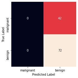
Polynomial Kernel

The Polynomial kernel is a non-stationary kernel. Polynomial kernels are well suited for problems where all the training data is normalized. In the case of this kernel, you also have to pass a value for the degree parameter of the SVC class. This basically is the degree of the polynomial.
Take a look at how we can use a polynomial kernel to implement kernel SVM:

clf = svm.SVC(kernel='poly', degree = 5, gamma = 100)
clf.fit(X_train, y_train)
y_predict = clf.predict(X_test)

print('Accuracy: ', metrics.accuracy_score(y_test, y_predict))

print('Precision: ', metrics.precision_score(y_test, y_predict))
print('Recall: ', metrics.recall_score(y_test, y_predict))

print('Confusion Matrix')

mat = metrics.confusion_matrix(y_test, y_predict)
sns.heatmap(mat, square = True, annot = True, fmt = 'd', cbar = False,
           xticklabels=cancer.target_names,
           yticklabels=cancer.target_names)

plt.xlabel('Predicted Label')
plt.ylabel('True Label')
plt.show()

Accuracy:  0.631578947368421
Precision:  0.631578947368421
Recall:  1.0
Confusion Matrix

Sigmoid Kernel

Finally, let's use a sigmoid kernel for implementing Kernel SVM.The sigmoid kernel was quite popular for support vector machines due to its origin from neural networks.To use the sigmoid kernel, you have to specify 'sigmoid' as value for the kernel parameter of the SVC class.
Take a look at the following script.

clf = svm.SVC(kernel='sigmoid', gamma = 200, C = 10000)
clf.fit(X_train, y_train)
y_predict = clf.predict(X_test)

print('Accuracy: ', metrics.accuracy_score(y_test, y_predict))

print('Precision: ', metrics.precision_score(y_test, y_predict))
print('Recall: ', metrics.recall_score(y_test, y_predict))

print('Confusion Matrix')

mat = metrics.confusion_matrix(y_test, y_predict)
sns.heatmap(mat, square = True, annot = True, fmt = 'd', cbar = False,
           xticklabels=cancer.target_names,
           yticklabels=cancer.target_names)

plt.xlabel('Predicted Label')
plt.ylabel('True Label')
plt.show()

Accuracy:  0.631578947368421
Precision:  0.631578947368421
Recall:  1.0
Confusion Matrix