One of the central concepts of data science is gaining insights from data. Statistics is an excellent tool for unlocking such insights in data. In this post, we’ll see some basic types of data(variable) which can be present in your dataset.

What is a Variable?

A variable is any characteristic, number, or quantity that can be measured or counted. They are called 'variables' because the value they take may vary, and it usually does. In programming, a variable is a value that can change, depending on conditions or on information passed to the program. The following are examples of variables:

• Age (21, 35, 62, ...)
• Gender (male, female)
• Income (GBP 20000, GBP 35000, GBP 45000, ...)
• House price (GBP 350000, GBP 570000, ...)
• Country of birth (China, Russia, Costa Rica, ...)
• Eye colour (brown, green, blue, ...)
• Vehicle make (Ford, Volkswagen, ...)

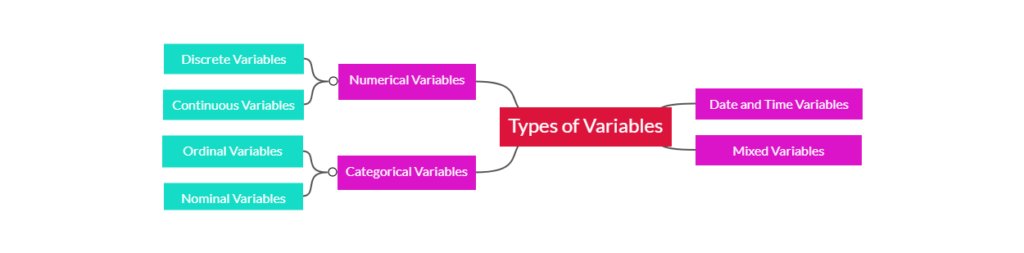
Most variables in a data set can be classified into one of four major types:

• Numerical variables
• Categorical variables
• Date-Time Variables
• Mixed Variables

Numeric Variables

The values of a numerical variable are numbers. They can be further classified into:

• Discrete variables
• Continuous variables

Discrete Variable

In a discrete variable, the values are whole numbers (counts). For example, the number of items bought by a customer in a supermarket is discrete. The customer can buy 1, 25, or 50 items, but not 3.7 items. It is always a round number. The following are examples of discrete variables:

• Number of active bank accounts of a borrower (1, 4, 7, ...)
• Number of pets in the family
• Number of children in the family

Continuous Variable

A variable that may contain any value within a range is continuous. For example, the total amount paid by a customer in a supermarket is continuous. The customer can pay, GBP 20.5, GBP 13.10, GBP 83.20 and so on. Other examples of continuous variables are:

• House price (in principle, it can take any value) (GBP 350000, 57000, 100000, ...)
• Time spent surfing a website (3.4 seconds, 5.10 seconds, ...)
• Total debt as percentage of total income in the last month (0.2, 0.001, 0, 0.75, ...)

Dataset

In this demo, we will use a toy data set which simulates data from a peer-to-peer finance company to inspect numerical and categorical variables.

• customer_id: Unique ID for each customer
• disbursed_amount: loan amount given to the borrower
• interest: interest rate
• income: annual income
• number_open_accounts: open accounts (more on this later)
• number_credit_lines_12: accounts opened in the last 12 months
• target: loan status(paid or being repaid = 1, defaulted = 0)
• loan_purpose: intended use of the loan
• market: the risk market assigned to the borrower (based in their financial situation)
• householder: whether the borrower owns or rents their property
• date_issued: date the loan was issued
• date_last_payment: date of last payment towards repyaing the loan

Let's start!

We will start by importing the necessary libraries.

• pandas is used to read the dataset into a dataframe and perform operations on it
• numpy is used to perform basic array operations
• pyplot from matplotlib is used to visualize the data

import pandas as pd
import numpy as np
import matplotlib.pyplot as plt

Now we will read the data using read_csv().  head() shows the first 5 rows of the dataframe.

data = pd.read_csv('https://raw.githubusercontent.com/laxmimerit/feature-engineering-for-machine-learning-dataset/master/loan.csv')
data.head()

	customer_id	disbursed_amount	interest	market	employment	time_employed	householder	income	date_issued	target	loan_purpose	number_open_accounts	date_last_payment	number_credit_lines_12
0	0	23201.5	15.4840	C	Teacher	<=5 years	RENT	84600.0	2013-06-11	0	Debt consolidation	4.0	2016-01-14	NaN
1	1	7425.0	11.2032	B	Accountant	<=5 years	OWNER	102000.0	2014-05-08	0	Car purchase	13.0	2016-01-25	NaN
2	2	11150.0	8.5100	A	Statistician	<=5 years	RENT	69840.0	2013-10-26	0	Debt consolidation	8.0	2014-09-26	NaN
3	3	7600.0	5.8656	A	Other	<=5 years	RENT	100386.0	2015-08-20	0	Debt consolidation	20.0	2016-01-26	NaN
4	4	31960.0	18.7392	E	Bus driver	>5 years	RENT	95040.0	2014-07-22	0	Debt consolidation	14.0	2016-01-11	NaN

Continuous Variables

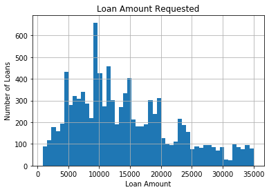
Let's look at the values of the variable disbursed_amount. It is the amount of money requested by the borrower. This variable is continuous and can take any principal value.

unique() method is used to know all type of unique values in the column. As we can see the values are not a whole number. They are continuous.

data['disbursed_amount'].unique()

array([23201.5 ,  7425.  , 11150.  , ...,  6279.  , 12894.75, 25584.  ])

To get a better idea we will visualize disbursed_amount by plotting a histogram. A histogram is an approximate representation of the distribution of numerical data.

To construct a histogram from a continuous variable you first need to split the data into intervals, called bins. A histogram displays numerical data by grouping data into "bins" of equal width. Each bin is plotted as a bar whose height corresponds to how many data points are in that bin. Here we are grouping the data into 50 different bins.

Notice that, there are no "gaps" between the bars (although some bars might be "absent" reflecting no frequencies). This is because a histogram represents a continuous variable, and as such, there are no gaps in the data. The values of the variable vary across the entire range of loan amounts typically disbursed to borrowers. This is characteristic of continuous variables.

fig = data['disbursed_amount'].hist(bins=50)

# title and axis labels
fig.set_title('Loan Amount Requested')
fig.set_xlabel('Loan Amount')
fig.set_ylabel('Number of Loans')

Now let's do the same exercise for the variable interest.It is the interest rate charged by the finance company to the borrowers. This variable is also continuous.

data['interest'].unique()

array([15.484 , 11.2032,  8.51  , ..., 12.9195, 11.2332, 11.0019])

Now we will plot a histogram.

fig = data['interest'].hist(bins=30)
fig.set_title('Interest Rate')
fig.set_xlabel('Interest Rate')
fig.set_ylabel('Number of Loans')

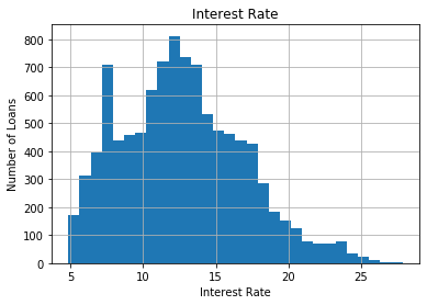
As there are no gaps in the histogram we can conclude that the values of the variable vary continuously across the variable range.

Now, let's explore the income declared by the customers, that is, how much they earn yearly. This variable is also continuous.

data['income'].unique()

array([ 84600.  , 102000.  ,  69840.  , ..., 228420.  , 133950.  ,
        55941.84])

Now let's plot the histogram.

fig = data['income'].hist(bins=100)

# For better visualisation, only specific range is displayed on the x-axis
fig.set_xlim(0, 400000)

# title and axis labels
fig.set_title("Customer's Annual Income")
fig.set_xlabel('Annual Income')
fig.set_ylabel('Number of Customers')

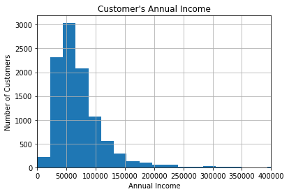
The majority of salaries are concentrated towards values in the range 30-70k, with only a few customers earning higher salaries. The value of the variable, varies continuously across the variable range, because this is a continuous variable.

Discrete Variables

Let's explore the variable "Number of open credit lines in the borrower's credit file" (number_open_accounts in the dataset). This variable represents the total number of credit items (credit cards, car loans, mortgages, etc.) that is known for that borrower. By definition it is a discrete variable, because a borrower can have 1 credit card, but not 3.5 credit cards.

data['number_open_accounts'].unique()

array([ 4., 13.,  8., 20., 14.,  5.,  9., 18., 16., 17., 12., 15.,  6.,
       10., 11.,  7., 21., 19., 26.,  2., 22., 27., 23., 25., 24., 28.,
        3., 30., 41., 32., 33., 31., 29., 37., 49., 34., 35., 38.,  1.,
       36., 42., 47., 40., 44., 43.])

# let's plot a histogram to get familiar with the distribution of the variable

fig = data['number_open_accounts'].hist(bins=100)

# for better visualisation, only specific range in the x-axis is displayed
fig.set_xlim(0, 30)

# title and axis labels
fig.set_title('Number of open accounts')
fig.set_xlabel('Number of open accounts')
fig.set_ylabel('Number of Customers')

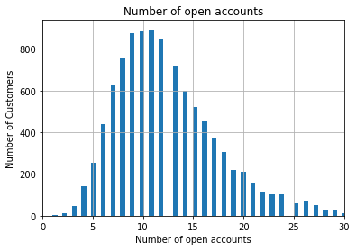
When the variables are discrete, gaps should be left between the bars. Histograms of discrete variables has this typical broken shape, as not all the values within the variable range are present in the variable. As mentioned earlier, the customer can have 3 credit cards, but not 3.5 credit cards.

Let's look at another example of a discrete variable in this dataset: Number of installment accounts opened in past 12 months(number_credit_lines_12 in the dataset).

Installment accounts are those, which at the moment of acquiring them, there is a set period and amount of repayments agreed between the lender and borrower. An example of this is a car loan, or a student loan. The borrower knows that they will pay a fixed amount over a fixed period, for example 36 months.

# let's inspect the variable values

data['number_credit_lines_12'].unique()

array([nan,  2.,  4.,  1.,  0.,  3.,  5.,  6.])

# let's make a histogram to get familiar with the distribution of the variable

fig = data['number_credit_lines_12'].hist(bins=50)

# title and axis labels
fig.set_title('Number of installment accounts opened in past 12 months')
fig.set_xlabel('Number of installment accounts opened in past 12 months')
fig.set_ylabel('Number of Borrowers')

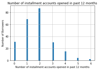
As the variable is discrete, you can observe the gaps between the bars. The majority of the borrowers have 1 or 2 installment accounts, with only a few borrowers having more than 2.

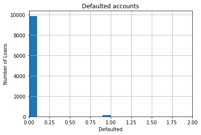
A variation of discrete variables: The binary variable

Binary variables, are discrete variables, that can take only 2 values(0 or 1, True or False, etc.), therefore they are called binary.

In our dataset target is a binary variable. It takes the values 0 or 1.

data['target'].unique()

array([0, 1], dtype=int64)

# let's make a histogram, although histograms for binary variables do not make a lot of sense

fig = data['target'].hist()

#only specific range in the x-axis is displayed
fig.set_xlim(0, 2)

# title and axis labels
fig.set_title('Defaulted accounts')
fig.set_xlabel('Defaulted')
fig.set_ylabel('Number of Loans')

Categorical Variable

A categorical variable is a variable that can take on one of a limited, and usually fixed, number of possible values. The values of a categorical variable are selected from a group of categories, also called labels. Examples are gender (male or female) and marital status (never married, married, divorced or widowed). Other examples of categorical variables include:

• Intended use of loan (debt-consolidation, car purchase, wedding expenses, ...)
• Mobile network provider (Vodafone, Orange, ...)
• Postcode

Categorical variables can be further categorised into:

• Ordinal Variables
• Nominal variables

Ordinal Variable

Ordinal variables are categorical variable in which the categories can be meaningfully ordered. For example:

• Student's grade in an exam (A, B, C or Fail).
• Days of the week, where Monday = 1 and Sunday = 7.
• Educational level, with the categories Elementary school, High school, College graduate and PhD ranked from 1 to 4.

Nominal Variable

For nominal variables, there isn't an intrinsic order in the labels. For example, country of birth, with values Argentina, England, Germany, etc., is nominal. Other examples of nominal variables include:

• Car colour (blue, grey, silver, ...)
• Vehicle make (Citroen, Peugeot, ...)
• City (Manchester, London, Chester, ...)

There is nothing that indicates an intrinsic order of the labels, and in principle, they are all equal.

Note:-

Sometimes categorical variables are coded as numbers when the data are recorded (e.g. gender may be coded as 0 for males and 1 for females). The variable is still categorical, despite the use of numbers.

In a similar way, individuals in a survey may be coded with a number that uniquely identifies them (maybe to avoid storing personal information for confidentiality). This number is really a label, and the variable is categorical. The number has no meaning other than making it possible to uniquely identify the observation (in this case the interviewed subject).

Ideally, when we work with a dataset in a business scenario, the data will come with a dictionary that indicates if the numbers in the variables are to be considered as categories or if they are numerical. And if the numbers are categories, the dictionary would explain what each value in the variable represents.

Let's inspect the variable householder, which indicates whether the borrowers own their homes or if they are renting, among other things. As you can see householder is a categorical(nominal) variable having 3 categories namely RENT, OWNER and MORTGAGE.

data['householder'].unique()

array(['RENT', 'OWNER', 'MORTGAGE'], dtype=object)

Now we will make a bar plot, with the number of loans for each category of home ownership the code below counts the number of observations (borrowers) of each category and then makes a bar plot.

fig = data['householder'].value_counts().plot.bar()
fig.set_title('Householder')
fig.set_ylabel('Number of customers')

Text(0, 0.5, 'Number of customers')

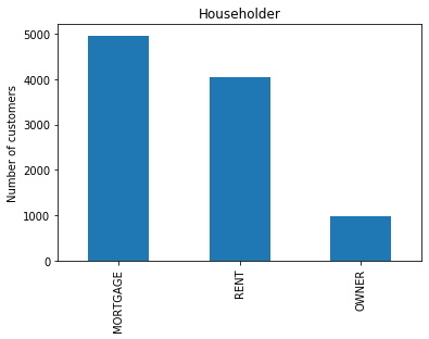
From the above bar plot we can infer that majority of the borrowers either own their house on a mortgage or rent their property. A few borrowers actually own their house. We can see the actual frequency of each category using value_counts().

data['householder'].value_counts()

MORTGAGE    4957
RENT        4055
OWNER        988
Name: householder, dtype: int64

The loan_purpose variable is another categorical(nominal) variable that indicates how the borrowers intend to use the money they are borrowing, for example to improve their house, or to cancel previous debt. Debt consolidation means that the borrower would like a loan to cancel previous debts, Car purchase means that the borrower is borrowing the money to buy a car, and so on. It gives an idea of the intended use of the loan.

data['loan_purpose'].unique()

array(['Debt consolidation', 'Car purchase', 'Other', 'Home improvements',
       'Moving home', 'Health', 'Holidays', 'Wedding'], dtype=object)

Let's make a bar plot with the number of borrowers within each category the code below counts the number of observations (borrowers) within each category and then makes a plot.

fig = data['loan_purpose'].value_counts().plot.bar()
fig.set_title('Loan Purpose')
fig.set_ylabel('Number of customers')

Text(0, 0.5, 'Number of customers')

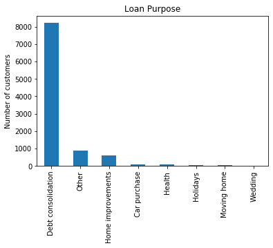
The majority of the borrowers intend to use the loan for debt consolidation. This is quite common. What the borrowers intend to do is, to consolidate all the debt that they have on different financial items, in one single debt which is the new loan that they will take from the peer to peer company. This loan will usually provide an advantage to the borrower, either in the form of lower interest rates than a credit card or longer repayment period.

Now we will look at one more categorical(ordinal) variable, market, which represents the risk market or risk band assigned to the borrower.

data['market'].unique()

array(['C', 'B', 'A', 'E', 'D'], dtype=object)

fig = data['market'].value_counts().plot.bar()
fig.set_title('Status of the Loan')
fig.set_ylabel('Number of customers')

Text(0, 0.5, 'Number of customers')

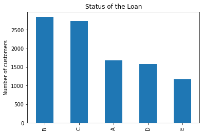
Most customers are assigned to markets B and C. A are lower risk customers, and E the highest risk customers. The higher the risk, the more likely the customer is to default, thus the finance companies charge higher interest rates on those loans.

Finally, let's look at a variable customer_id that is numerical, but its numbers have no real meaning. Their values are more like "labels" than real numbers.

data['customer_id'].head()

0    0
1    1
2    2
3    3
4    4
Name: customer_id, dtype: int64

The variable has as many different id values as customers, in this case 10000.

len(data['customer_id'].unique())

10000

Each id represents one customer. This number is assigned to identify the customer if needed, while maintaining confidentiality and ensuring data protection.

Dates and Times

A special type of categorical variable are those that instead of taking traditional labels, like color (blue, red), or city (London, Manchester), take dates and / or time as values. For example, date of birth ('29-08-1987', '12-01-2012'), or date of application ('2016-Dec', '2013-March').

Datetime variables can contain dates only, time only, or date and time.

We don't usually work with a datetime variable in their raw format because:

• Date variables contain a huge number of different categories
• We can extract much more information from datetime variables by preprocessing them correctly

In addition, often, date variables will contain dates that were not present in the dataset used to train the machine learning model. In fact, date variables will usually contains dates from the future, respect to the dates in the training dataset. Therefore, the machine learning model will not know what to do with them, because it never saw them while being trained.

pandas assigns type object when reading dates and considers them as strings.

data[['date_issued', 'date_last_payment']].dtypes

date_issued          object
date_last_payment    object
dtype: object

Both date_issued and date_last_payment are casted as objects. Therefore, pandas will treat them as strings or categorical variables. In order to instruct pandas to treat them as dates, we need to re-cast them into datetime format. Here we will parse the dates, currently coded as strings, into datetime format this will allow us to make some analysis afterwards. The new formatted dates are stored in date_issued_dt and date_last_payment_dt.

data['date_issued_dt'] = pd.to_datetime(data['date_issued'])
data['date_last_payment_dt'] = pd.to_datetime(data['date_last_payment'])
data[['date_issued', 'date_issued_dt', 'date_last_payment', 'date_last_payment_dt']].head()

	date_issued	date_issued_dt	date_last_payment	date_last_payment_dt
0	2013-06-11	2013-06-11	2016-01-14	2016-01-14
1	2014-05-08	2014-05-08	2016-01-25	2016-01-25
2	2013-10-26	2013-10-26	2014-09-26	2014-09-26
3	2015-08-20	2015-08-20	2016-01-26	2016-01-26
4	2014-07-22	2014-07-22	2016-01-11	2016-01-11

data[['date_issued_dt', 'date_last_payment_dt']].dtypes

date_issued_dt          datetime64[ns]
date_last_payment_dt    datetime64[ns]
dtype: object

Now we will extract the month and the year from the date into month and year respectively to make better plots.

data['month'] = data['date_issued_dt'].dt.month
data['year'] = data['date_issued_dt'].dt.year

Let's see how much money Lending Club has disbursed (i.e. lent) over the years to the different risk markets (grade variable). We will group the data according to the year, month and market. unstack() function in dataframe unstacks the row to columns .

fig = data.groupby(['year','month', 'market'])['disbursed_amount'].sum().unstack().plot(
    figsize=(14, 8), linewidth=2)

fig.set_title('Disbursed amount in time')
fig.set_ylabel('Disbursed Amount')

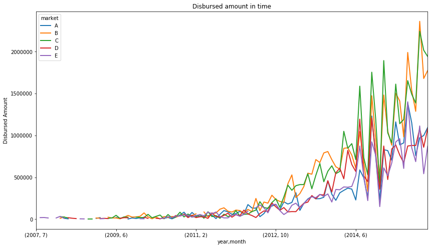
This toy finance company seems to have increased the amount of money lent from 2012 onwards. The tendency indicates that they continue to grow. In addition, we can see that their major business comes from lending money to C and B grades.

A grades are the lower risk borrowers, borrowers that most likely will be able to repay their loans, as they are typically in a better financial situation. Borrowers within this grade are charged lower interest rates.

D and E grades represent the riskier borrowers. Usually borrowers in somewhat tighter financial situations, or for whom there is not sufficient financial history to make a reliable credit assessment. They are typically charged higher rates, as the business, and therefore the investors, take a higher risk when lending them money.

Mixed Variables

Mixed variables are those which values contain both numbers and labels.

Variables can be mixed for a variety of reasons. For example, when credit agencies gather and store financial information of users, usually, the values of the variables they store are numbers. However, in some cases the credit agencies cannot retrieve information for a certain user for different reasons. What Credit Agencies do in these situations is to code each different reason due to which they failed to retrieve information with a different code or 'label'. While doing so they generate mixed type variables. These variables contain numbers when the value could be retrieved, or labels otherwise.

As an example, think of the variable number_of_open_accounts. It can take any number, representing the number of different financial accounts of the borrower. Sometimes, information may not be available for a certain borrower, for a variety of reasons. Each reason will be coded by a different letter, for example: 'A': couldn't identify the person, 'B': no relevant data, 'C': person seems not to have any open account.

Another example of mixed type variables, is for example the variable missed_payment_status. This variable indicates, whether a borrower has missed a (any) payment in their financial item. For example, if the borrower has a credit card, this variable indicates whether they missed a monthly payment on it. Therefore, this variable can take values of 0, 1, 2, 3 meaning that the customer has missed 0-3 payments in their account. And it can also take the value D, if the customer defaulted on that account. Typically, once the customer has missed 3 payments, the lender declares the item defaulted (D), that is why this variable takes numerical values 0-3 and then D.

Dataset

The dataset used to study Mixed Variables contains 2 columns id and open_il_24m. id is the unique key for each borrower and open_il_24m is the number of installment accounts opened in past 24 months by that borrower. Installment accounts are those that, at the moment of acquiring them, there is a set period and amount of repayments agreed between the lender and borrower. An example of this is a car loan, or a student loan. The borrowers know that they are going to pay a fixed amount over a fixed period.

We will begin by reading the dataset into a dataframe.

data = pd.read_csv('https://raw.githubusercontent.com/laxmimerit/feature-engineering-for-machine-learning-dataset/master/sample_s2.csv')
data.head()

	id	open_il_24m
0	1077501	C
1	1077430	A
2	1077175	A
3	1076863	A
4	1075358	A

The data contains 887379 rows and 2 columns.

data.shape

(887379, 2)

Fictitious meaning of the different letters / codes in the variable open_il_24m are:

• 'A': couldn't identify the person
• 'B': no relevant data
• 'C': person seems not to have any account open

Let's see all the unique values the variable contained by the variable.

data.open_il_24m.unique()

array(['C', 'A', 'B', '0.0', '1.0', '2.0', '4.0', '3.0', '6.0', '5.0',
       '9.0', '7.0', '8.0', '13.0', '10.0', '19.0', '11.0', '12.0',
       '14.0', '15.0'], dtype=object)

Here we are displaying the frequency of these unique values.

data.open_il_24m.value_counts()

A       500548
C       300000
B        65459
1.0       6436
0.0       5481
2.0       4448
3.0       2468
4.0       1249
5.0        606
6.0        309
7.0        163
8.0         81
9.0         47
10.0        28
11.0        23
12.0        17
13.0         7
14.0         6
15.0         2
19.0         1
Name: open_il_24m, dtype: int64

Now we will make a bar plot showing the different number of borrowers for each of the values of the mixed variable.

fig = data.open_il_24m.value_counts().plot.bar()
fig.set_title('Number of installment accounts open')
fig.set_ylabel('Number of borrowers')

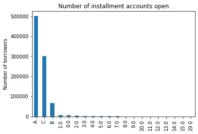
This is how a mixed variable looks like!

Summary