Watch Full Playlist: https://www.youtube.com/playlist?list=PLc2rvfiptPSQYzmDIFuq2PqN2n28ZjxDH

Linear Regression

Let’s first understand what exactly linear regression is, it is a straight forward approach to predict the response y on the basis of different prediction variables such x and ε. . There is a linear relation between x and y.

𝑦𝑖 = 𝛽0 + 𝛽1.𝑋𝑖 + 𝜀𝑖

y = dependent variable
β0 = population of intercept
βi = population of co-efficient
x = independent variable
εi= Random error

Basic Assumptions

• Linear relationship with the target y
• Feature space X should have gaussian distribution
• Features are not correlated with other
• Features are in same scale i.e. have same variance

Lasso (L1) and Ridge (L2) Regularization

Regularization is a technique to discourage the complexity of the model. It does this by penalizing the loss function. This helps to solve the overfitting problem.

• L1 regularization (also called Lasso)
  It shrinks the co-efficients which are less important to zero. That means with Lasso regularization we can remove some features.
• L2 regularization (also called Ridge)
  It does’t reduce the co-efficients to zero but it reduces the regression co-efficients with this reduction we can identofy which feature has more important.
• L1/L2 regularization (also called Elastic net)

A regression model that uses L1 regularization technique is called Lasso Regression and model which uses L2 is called Ridge Regression.

What is Lasso Regularisation

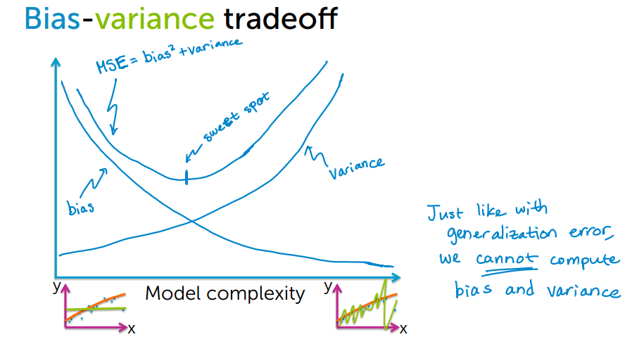
3 sources of error

• Noise:
  We can’t do anything with the noise. Let’s focus on following errors.
• Bias error:
  It is useful to quantify how much on an average are the predicted values different from the actual value.
• Variance:
  On the other side quantifies how are the prediction made on the same observation different from each other.

Now we will try to understand bias - variance trade off from the following figure.
By increasing model complexity, total error will decrease till some point and then it will start to increase. W need to select optimum model complexity to get less error.

If you are getting high bias then you have a fair chance to increase model complexity. And otherside it you are getting high variance, you need to decrease model complexity that’s how any machine learning algorithm works.

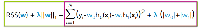
The L1 regularization adds a penalty equal to the sum of the absolute value of the coefficients.

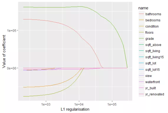
We can observe from the following figure. The L1 regularization will shrink some parameters to zero. Hence some variables will not play any role in the model to get final output, L1 regression can be seen as a way to select features in a model.

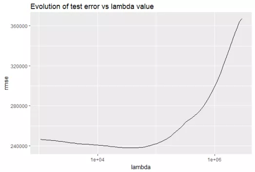
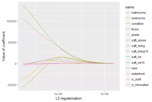
Let’s observe the evolution of test error by changing the value of λ from the following figure.

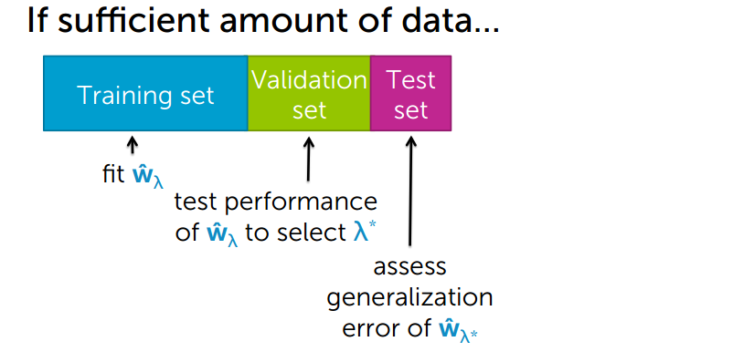
How to choose λ

Let’s move ahead and choose the best λ.

We have a sufficient amount of data. In that we can split our data into 3 sets those are

• Training set
• Validation set
• Test set

• In the training set, we fit our model and set regression co-efficients with the regularization.
• Then we test our model’s performance to select λ

• on validation set, if any thing wrong with the model like less accuracy we validate on the validation set then we change the parameter the we go back to the training set and so the optimization.
• Finally, it will do generalize testing on the test set.

What is Ridge Regularisation

Let’s first understand what exactly Ridge regularization:

The L2 regularization adds a penalty equal to the sum of the squared value of the coefficients.

λ is the tuning parameter or optimization parameter.
w is the regression co-efficient.

In this regularization,
if λ is high then we will get high bias and low variance.
if λ is low then we will get low bias and high variance

So what we do we will find out the optimized value of λ by tuning the parameters. And we can say λ is the strength of the regularization.

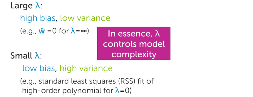
The L2 regularization will force the parameters to be relatively small, the bigger the penalization, the smaller (and the more robust) the coefficients are.

Difference between L1 and L2 regularization

Let’s discuss the difference between L1 and L2 regularization:

L1 Regularization	L2 Regularization
It penalizes sum of absolute value of weights	It regularization penalizes sum of square weights
It has a sparse solution	It has a non sparse solution
It has multiple solutions	It has one solution
It has built in feature selection	It has no feature selection
It is robust to outliers	It is not robust to outliers
It generates model that are simple and interpretable but cannot learn complex patterns	It gives better prediction when output variable is a function of all input features

Load the dataset

Loading required libraries

import numpy as np
import pandas as pd
import seaborn as sns
import matplotlib.pyplot as plt
%matplotlib inline

from sklearn.model_selection import train_test_split
from sklearn.ensemble import RandomForestClassifier
from sklearn.feature_selection import SelectKBest, SelectPercentile
from sklearn.metrics import accuracy_score

from sklearn.linear_model import LinearRegression, LogisticRegression
from sklearn.feature_selection import SelectFromModel

titanic = sns.load_dataset('titanic')
titanic.head()

	survived	pclass	sex	age	sibsp	parch	fare	embarked	class	who	adult_male	deck	embark_town	alive	alone
0	0	3	male	22.0	1	0	7.2500	S	Third	man	True	NaN	Southampton	no	False
1	1	1	female	38.0	1	0	71.2833	C	First	woman	False	C	Cherbourg	yes	False
2	1	3	female	26.0	0	0	7.9250	S	Third	woman	False	NaN	Southampton	yes	True
3	1	1	female	35.0	1	0	53.1000	S	First	woman	False	C	Southampton	yes	False
4	0	3	male	35.0	0	0	8.0500	S	Third	man	True	NaN	Southampton	no	True

titanic.isnull().sum()

survived         0
pclass           0
sex              0
age            177
sibsp            0
parch            0
fare             0
embarked         2
class            0
who              0
adult_male       0
deck           688
embark_town      2
alive            0
alone            0
dtype: int64

Let’s remove age and deck from the feature list

titanic.drop(labels = ['age', 'deck'], axis = 1, inplace = True)
titanic = titanic.dropna()
titanic.isnull().sum()

survived       0
pclass         0
sex            0
sibsp          0
parch          0
fare           0
embarked       0
class          0
who            0
adult_male     0
embark_town    0
alive          0
alone          0
dtype: int64

Let’s get the features of the data

data = titanic[['pclass', 'sex', 'sibsp', 'parch', 'embarked', 'who', 'alone']].copy()
data.head()

	pclass	sex	sibsp	parch	embarked	who	alone
0	3	male	1	0	S	man	False
1	1	female	1	0	C	woman	False
2	3	female	0	0	S	woman	True
3	1	female	1	0	S	woman	False
4	3	male	0	0	S	man	True

data.isnull().sum()

pclass      0
sex         0
sibsp       0
parch       0
embarked    0
who         0
alone       0
dtype: int64

sex = {'male': 0, 'female': 1}
data['sex'] = data['sex'].map(sex)
data.head()

	pclass	sex	sibsp	parch	embarked	who	alone
0	3	0	1	0	S	man	False
1	1	1	1	0	C	woman	False
2	3	1	0	0	S	woman	True
3	1	1	1	0	S	woman	False
4	3	0	0	0	S	man	True

ports = {'S': 0, 'C': 1, 'Q': 2}
data['embarked'] = data['embarked'].map(ports)
who = {'man': 0, 'woman': 1, 'child': 2}
data['who'] = data['who'].map(who)
alone = {True: 1, False: 0}
data['alone'] = data['alone'].map(alone)
data.head()

	pclass	sex	sibsp	parch	embarked	who	alone
0	3	0	1	0	0	0	0
1	1	1	1	0	1	1	0
2	3	1	0	0	0	1	1
3	1	1	1	0	0	1	0
4	3	0	0	0	0	0	1

Let’s read the data into x

X = data.copy()
y = titanic['survived']
X.shape, y.shape

((889, 7), (889,))

X_train, X_test, y_train, y_test = train_test_split(X, y, test_size = 0.3, random_state = 43)

Estimation of coefficients of Linear Regression

First we will go with estimation of coefficients of linear regression

sel = SelectFromModel(LinearRegression())

Let’s go ahead and fit the model

sel.fit(X_train, y_train)
SelectFromModel(estimator=LinearRegression(copy_X=True, fit_intercept=True, n_jobs=None,
         normalize=False),
        max_features=None, norm_order=1, prefit=False, threshold=None)

With these we have trained our model

Let’s see the features of the model

sel.get_support()

array([ True,  True, False, False, False,  True, False])

Now we will try to get the co-efficients

sel.estimator_.coef_

array([-0.13750402,  0.26606466, -0.07470416, -0.0668525 ,  0.04793674,
        0.23857799, -0.12929595])

Let’s get the mean of the co-efficients

mean = np.mean(np.abs(sel.estimator_.coef_))
mean

0.13727657291370804

And calculate the absolute value of the co-efficients

np.abs(sel.estimator_.coef_)

array([0.13750402, 0.26606466, 0.07470416, 0.0668525 , 0.04793674,
       0.23857799, 0.12929595])

features = X_train.columns[sel.get_support()]
features

Index(['pclass', 'sex', 'who'], dtype='object')

Let’s get the transformed version of x_train and x_test.

X_train_reg = sel.transform(X_train)
X_test_reg = sel.transform(X_test)
X_test_reg.shape

(267, 3)

Let’s implement the randomForest function and we wil do the training of the model.

def run_randomForest(X_train, X_test, y_train, y_test):
    clf = RandomForestClassifier(n_estimators=100, random_state=0, n_jobs=-1)
    clf = clf.fit(X_train, y_train)
    y_pred = clf.predict(X_test)
    print('Accuracy: ', accuracy_score(y_test, y_pred))

%%time
run_randomForest(X_train_reg, X_test_reg, y_train, y_test)

Accuracy:  0.8239700374531835
Wall time: 250 ms

Now we will get the accuracy and wall time on the original data set

%%time
run_randomForest(X_train, X_test, y_train, y_test)

Accuracy:  0.8239700374531835
Wall time: 252 ms

X_train.shape

(622, 7)

Logistic Regression Coefficient with L1 Regularization

Let’s move ahead with the L1 regularization to select the features.

sel = SelectFromModel(LogisticRegression(penalty = 'l1', C = 0.05, solver = 'liblinear'))
sel.fit(X_train, y_train)
sel.get_support()

array([ True,  True,  True, False, False,  True, False])

Let’s get the regression co-efficients.

sel.estimator_.coef_

array([[-0.54045394, 0.78039608, -0.14081954, 0., 0.        ,0.94106713, 0.]])

Let’s get the transformed version of x_train and x_test by using the function transform()

X_train_l1 = sel.transform(X_train)
X_test_l1 = sel.transform(X_test)

Now we will get the accuracy

%%time
run_randomForest(X_train_l1, X_test_l1, y_train, y_test)

Accuracy:  0.8277153558052435
Wall time: 251 ms

L2 Regularization

Let’s move ahead with the L2 regularization to select the features.

sel = SelectFromModel(LogisticRegression(penalty = 'l2', C = 0.05, solver = 'liblinear'))
sel.fit(X_train, y_train)
sel.get_support()

array([ True,  True, False, False, False,  True, False])

sel.estimator_.coef_

array([[-0.55749685,  0.85692344, -0.30436065, -0.11841967,  0.2435823 ,
         1.00124155, -0.29875898]])

X_train_l1 = sel.transform(X_train)
X_test_l1 = sel.transform(X_test)

Let’s check the accuracy of the data

%%time
run_randomForest(X_train_l1, X_test_l1, y_train, y_test)

Accuracy:  0.8239700374531835
Wall time: 250 ms