Feature Selection Based on Mutual Information (Entropy) Gain for Classification and Regression | Machine Learning | KGP Talkie
Feature Selection Based on Mutual Information (Entropy) Gain
Watch Full Playlist: https://www.youtube.com/playlist?list=PLc2rvfiptPSQYzmDIFuq2PqN2n28ZjxDH
What is Mutual Information
The elimination process aims to reduce the size of the input feature set and at the same time to retain the class discriminatory information for classification problems.
Mutual information (MI) is a measure of the amount of information between two random variables is symmetric and non-negative, and it could be zero if and only if the variables are independent.
It is NP hard optimization problem in computer science branch. The best approach which we in general follow is greedy solution for feature selection. Those approaches are step-wise forward feature selection or step-wise backward feature selection.
Classification Problem
Dataset Available at: https://github.com/laxmimerit/Data-Files-for-Feature-Selection
Importing required libraries
import numpy as np
import pandas as pd
import matplotlib.pyplot as plt
import seaborn as sns
from sklearn.model_selection import train_test_split
from sklearn.ensemble import RandomForestClassifier
from sklearn.metrics import accuracy_score
from sklearn.feature_selection import VarianceThreshold, mutual_info_classif, mutual_info_regression
from sklearn.feature_selection import SelectKBest, SelectPercentile
Let’s read the data into the variable data.
data = pd.read_csv('train.csv', nrows = 20000)
data.head()
| ID | var3 | var15 | imp_ent_var16_ult1 | imp_op_var39_comer_ult1 | imp_op_var39_comer_ult3 | imp_op_var40_comer_ult1 | imp_op_var40_comer_ult3 | imp_op_var40_efect_ult1 | imp_op_var40_efect_ult3 | … | saldo_medio_var33_hace2 | saldo_medio_var33_hace3 | saldo_medio_var33_ult1 | saldo_medio_var33_ult3 | saldo_medio_var44_hace2 | saldo_medio_var44_hace3 | saldo_medio_var44_ult1 | saldo_medio_var44_ult3 | var38 | TARGET | |
|---|---|---|---|---|---|---|---|---|---|---|---|---|---|---|---|---|---|---|---|---|---|
| 0 | 1 | 2 | 23 | 0.0 | 0.0 | 0.0 | 0.0 | 0.0 | 0 | 0 | … | 0.0 | 0.0 | 0.0 | 0.0 | 0.0 | 0.0 | 0.0 | 0.0 | 39205.170000 | 0 |
| 1 | 3 | 2 | 34 | 0.0 | 0.0 | 0.0 | 0.0 | 0.0 | 0 | 0 | … | 0.0 | 0.0 | 0.0 | 0.0 | 0.0 | 0.0 | 0.0 | 0.0 | 49278.030000 | 0 |
| 2 | 4 | 2 | 23 | 0.0 | 0.0 | 0.0 | 0.0 | 0.0 | 0 | 0 | … | 0.0 | 0.0 | 0.0 | 0.0 | 0.0 | 0.0 | 0.0 | 0.0 | 67333.770000 | 0 |
| 3 | 8 | 2 | 37 | 0.0 | 195.0 | 195.0 | 0.0 | 0.0 | 0 | 0 | … | 0.0 | 0.0 | 0.0 | 0.0 | 0.0 | 0.0 | 0.0 | 0.0 | 64007.970000 | 0 |
| 4 | 10 | 2 | 39 | 0.0 | 0.0 | 0.0 | 0.0 | 0.0 | 0 | 0 | … | 0.0 | 0.0 | 0.0 | 0.0 | 0.0 | 0.0 | 0.0 | 0.0 | 117310.979016 | 0 |
5 rows × 371 columns
X = data.drop('TARGET', axis = 1)
y = data['TARGET']
X.shape, y.shape
((20000, 370), (20000,))
Let’s go ahead and train , test and split the dataset.
X_train, X_test, y_train, y_test = train_test_split(X, y, test_size = 0.2, random_state = 0, stratify = y)
Remove constant, quasi constant, and duplicate features
These are the filters that are almost constant or quasi constant in other words these features have same values for large subset of outputs and such features are not very useful for making predictions.
There is no rule for fixing threshold value but generally we can take as 99% similarity and 1% of non similarity.
Let’s go ahead see how many quasi constant features are there.
constant_filter = VarianceThreshold(threshold=0.01)
constant_filter.fit(X_train)
X_train_filter = constant_filter.transform(X_train)
X_test_filter = constant_filter.transform(X_test)
Let’s transpose the dataset training and testing dataset.
X_train_T = X_train_filter.T
X_test_T = X_test_filter.T
X_train_T = pd.DataFrame(X_train_T)
X_test_T = pd.DataFrame(X_test_T)
Let’s get the total number of duplicated rows.
X_train_T.duplicated().sum()
18
duplicated_features = X_train_T.duplicated()
Let’s get the non-duplicated features.
features_to_keep = [not index for index in duplicated_features]
X_train_unique = X_train_T[features_to_keep].T
X_test_unique = X_test_T[features_to_keep].T
X_train_unique.shape, X_test_unique.shape
((16000, 227), (4000, 227))
Now, we can observe here out of 370 we have only 227 features.
Calculate the MI
Let’s calculate the mutual information among the 227 features.
mutual_info_classif( )
Mutual information measures the dependency between the variables. It is equal to zero if and only if two random variables are independent, and higher values mean higher dependency.
mi = mutual_info_classif(X_train_unique, y_train)
len(mi)
227
mi[: 10]
array([0.0025571 , 0.        , 0.01479401, 0.        , 0.        ,
       0.00133223, 0.        , 0.        , 0.00197431, 0.        ])
mi = pd.Series(mi) mi.index = X_train_unique.columns
Let’s sort the values in the descending order.
mi.sort_values(ascending=False, inplace = True)
Let’s observe the Mutual Information with respect to features from following bar plot.
plt.title('Mutual information with respect to features')
mi.plot.bar(figsize = (16,5))
plt.show()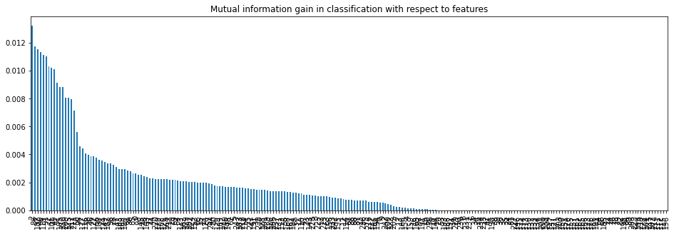
Let’s go ahead and work with percentile. We will select 10 percentile of the features. Let’s have a look at following code.
sel = SelectPercentile(mutual_info_classif, percentile=10).fit(X_train_unique, y_train)
X_train_unique.columns[sel.get_support()]
Int64Index([  2,  22,  40,  49,  50,  51,  52,  61,  86,  91,  98, 100, 101,
            105, 119, 125, 127, 182, 187, 209, 210, 211, 212],
           dtype='int64')
len(X_train_unique.columns[sel.get_support()])
23
Let’s transform the training and testing dataset. Let’s have a look at the following code.
X_train_mi = sel.transform(X_train_unique)
X_test_mi = sel.transform(X_test_unique)
X_train_mi.shape
(16000, 23)
Build the model and compare the performance
Let’s apply the Random forest classifier with number of estimators equals to 100. And then predict the y values by using tesung dataset.
def run_randomForest(X_train, X_test, y_train, y_test):
    clf = RandomForestClassifier(n_estimators=100, random_state=0, n_jobs=-1)
    clf.fit(X_train, y_train)
    y_pred = clf.predict(X_test)
    print('Accuracy on test set: ')
    print(accuracy_score(y_test, y_pred))
Now will calculate the accuarcy and traing time of trined dataset.
%%time
run_randomForest(X_train_mi, X_test_mi, y_train, y_test)
Accuracy on test set:
0.95825
Wall time: 1.14 s
Now will calculate the accuarcy and traing time of trined dataset.
%%time
run_randomForest(X_train, X_test, y_train, y_test)
Accuracy on test set:
0.9585
Wall time: 2.41 s
(1.46-0.57)*100/1.46
60.95890410958904
Mutual Information Gain in Regression
from sklearn.datasets import load_boston
from sklearn.linear_model import LinearRegression
from sklearn.metrics import mean_absolute_error, mean_squared_error, r2_score
Load boston dataset into the variable boston.
boston = load_boston()
print(boston.DESCR)
.. _boston_dataset:

Boston house prices dataset
---------------------------

**Data Set Characteristics:**

    :Number of Instances: 506

    :Number of Attributes: 13 numeric/categorical predictive. Median Value (attribute 14) is usually the target.

    :Attribute Information (in order):
        - CRIM     per capita crime rate by town
        - ZN       proportion of residential land zoned for lots over 25,000 sq.ft.
        - INDUS    proportion of non-retail business acres per town
        - CHAS     Charles River dummy variable (= 1 if tract bounds river; 0 otherwise)
        - NOX      nitric oxides concentration (parts per 10 million)
        - RM       average number of rooms per dwelling
        - AGE      proportion of owner-occupied units built prior to 1940
        - DIS      weighted distances to five Boston employment centres
        - RAD      index of accessibility to radial highways
        - TAX      full-value property-tax rate per $10,000
        - PTRATIO  pupil-teacher ratio by town
        - B        1000(Bk - 0.63)^2 where Bk is the proportion of blacks by town
        - LSTAT    % lower status of the population
        - MEDV     Median value of owner-occupied homes in $1000's

    :Missing Attribute Values: None

    :Creator: Harrison, D. and Rubinfeld, D.L.

This is a copy of UCI ML housing dataset.
https://archive.ics.uci.edu/ml/machine-learning-databases/housing/


This dataset was taken from the StatLib library which is maintained at Carnegie Mellon University.

The Boston house-price data of Harrison, D. and Rubinfeld, D.L. 'Hedonic
prices and the demand for clean air', J. Environ. Economics & Management,
vol.5, 81-102, 1978.   Used in Belsley, Kuh & Welsch, 'Regression diagnostics
...', Wiley, 1980.   N.B. Various transformations are used in the table on
pages 244-261 of the latter.

The Boston house-price data has been used in many machine learning papers that address regression
problems.
X = pd.DataFrame(data = boston.data, columns=boston.feature_names) X.head()
| CRIM | ZN | INDUS | CHAS | NOX | RM | AGE | DIS | RAD | TAX | PTRATIO | B | LSTAT | |
|---|---|---|---|---|---|---|---|---|---|---|---|---|---|
| 0 | 0.00632 | 18.0 | 2.31 | 0.0 | 0.538 | 6.575 | 65.2 | 4.0900 | 1.0 | 296.0 | 15.3 | 396.90 | 4.98 |
| 1 | 0.02731 | 0.0 | 7.07 | 0.0 | 0.469 | 6.421 | 78.9 | 4.9671 | 2.0 | 242.0 | 17.8 | 396.90 | 9.14 |
| 2 | 0.02729 | 0.0 | 7.07 | 0.0 | 0.469 | 7.185 | 61.1 | 4.9671 | 2.0 | 242.0 | 17.8 | 392.83 | 4.03 |
| 3 | 0.03237 | 0.0 | 2.18 | 0.0 | 0.458 | 6.998 | 45.8 | 6.0622 | 3.0 | 222.0 | 18.7 | 394.63 | 2.94 |
| 4 | 0.06905 | 0.0 | 2.18 | 0.0 | 0.458 | 7.147 | 54.2 | 6.0622 | 3.0 | 222.0 | 18.7 | 396.90 | 5.33 |
y = boston.target
Now, train, test and split the dataset with test size equals to 0.2.
X_train, X_test, y_train, y_test = train_test_split(X, y, test_size = 0.2, random_state = 0)
mi = mutual_info_regression(X_train, y_train)
mi = pd.Series(mi)
mi.index = X_train.columns
mi.sort_values(ascending=False, inplace = True)
mi
LSTAT      0.676729
RM         0.557777
INDUS      0.504754
PTRATIO    0.492141
NOX        0.445376
TAX        0.373128
CRIM       0.349371
AGE        0.347299
DIS        0.321057
RAD        0.203106
ZN         0.201467
B          0.152778
CHAS       0.008383
dtype: float64
plt.title('Mutual information with respect to features')
mi.plot.bar()
plt.show()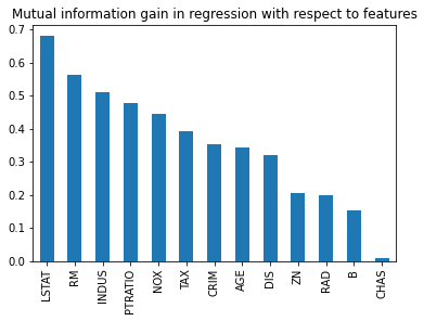
sel = SelectKBest(mutual_info_regression, k = 9).fit(X_train, y_train)
X_train.columns[sel.get_support()]
Index(['CRIM', 'INDUS', 'NOX', 'RM', 'AGE', 'DIS', 'TAX', 'PTRATIO', 'LSTAT'], dtype='object')
Let’s apply Linear regression function and find out the predicted value of y.
model = LinearRegression()
model.fit(X_train, y_train)
y_predict = model.predict(X_test)
r2_score(y_test, y_predict)
0.5892223849182507
Let’s calculate the RMS error value.
np.sqrt(mean_squared_error(y_test, y_predict))
5.783509315085146
Let’s get the standard deviation of y.
np.std(y)
9.188011545278203
Let’s transform the trained dataset.
X_train_9 = sel.transform(X_train)
X_train_9.shape
(404, 9)
X_test_9 = sel.transform(X_test)
model = LinearRegression()
model.fit(X_train_9, y_train)
y_predict = model.predict(X_test_9)
print('r2_score')
r2_score(y_test, y_predict)
r2_score
0.5317127606961576
Let’s calculate the RMS error value.
print('rmse')
np.sqrt(mean_squared_error(y_test, y_predict))
rmse 6.175103151293747
0 Comments