Feature Selection Based on Univariate (ANOVA) Test for Classification

Watch Full Playlist: https://www.youtube.com/playlist?list=PLc2rvfiptPSQYzmDIFuq2PqN2n28ZjxDH

What is Univariate (ANOVA) Test

The elimination process aims to reduce the size of the input feature set and at the same time to retain the class discriminatory information for classification problems.

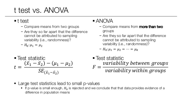
An F-test is any statistical test in which the test statistic has an F-distribution under the null hypothesis.

Analysis of variance (ANOVA) is a collection of statistical models and their associated estimation procedures (such as the "variation" among and between groups) used to analyze the differences among group means in a sample.

The F-test is used for comparing the factors of the total deviation. For example, in one-way, or single-factor ANOVA, statistical significance is tested for by comparing the F test statistic

Classification Problem

Importing required libraries

import numpy as np
import pandas as pd
import matplotlib.pyplot as plt
import seaborn as sns

from sklearn.model_selection import train_test_split
from sklearn.ensemble import RandomForestClassifier
from sklearn.metrics import accuracy_score
from sklearn.feature_selection import VarianceThreshold
from sklearn.feature_selection import f_classif, f_regression
from sklearn.feature_selection import SelectKBest, SelectPercentile

Download DataFiles: https://github.com/laxmimerit/Data-Files-for-Feature-Selection

data = pd.read_csv('train.csv', nrows = 20000)
data.head()

	ID	var3	var15	imp_ent_var16_ult1	imp_op_var39_comer_ult1	imp_op_var39_comer_ult3	imp_op_var40_comer_ult1	imp_op_var40_comer_ult3	imp_op_var40_efect_ult1	imp_op_var40_efect_ult3	...	saldo_medio_var33_hace2	saldo_medio_var33_hace3	saldo_medio_var33_ult1	saldo_medio_var33_ult3	saldo_medio_var44_hace2	saldo_medio_var44_hace3	saldo_medio_var44_ult1	saldo_medio_var44_ult3	var38	TARGET
0	1	2	23	0.0	0.0	0.0	0.0	0.0	0	0	...	0.0	0.0	0.0	0.0	0.0	0.0	0.0	0.0	39205.170000	0
1	3	2	34	0.0	0.0	0.0	0.0	0.0	0	0	...	0.0	0.0	0.0	0.0	0.0	0.0	0.0	0.0	49278.030000	0
2	4	2	23	0.0	0.0	0.0	0.0	0.0	0	0	...	0.0	0.0	0.0	0.0	0.0	0.0	0.0	0.0	67333.770000	0
3	8	2	37	0.0	195.0	195.0	0.0	0.0	0	0	...	0.0	0.0	0.0	0.0	0.0	0.0	0.0	0.0	64007.970000	0
4	10	2	39	0.0	0.0	0.0	0.0	0.0	0	0	...	0.0	0.0	0.0	0.0	0.0	0.0	0.0	0.0	117310.979016	0

5 rows × 371 columns

X = data.drop('TARGET', axis = 1)
y = data['TARGET']
X.shape, y.shape

((20000, 370), (20000,))

Now train, test and split the data with test size equals to 0.2.

X_train, X_test, y_train, y_test = train_test_split(X, y, test_size = 0.2, random_state = 0, stratify = y)

Remove Constant, Quasi Constant, and Correlated Features

These are the filters that are almost constant or quasi constant in other words these features have same values for large subset of outputs and such features are not very useful for making predictions

Let's remove the constant and quasi constant features with the following code.

constant_filter = VarianceThreshold(threshold=0.01)
constant_filter.fit(X_train)
X_train_filter = constant_filter.transform(X_train)
X_test_filter = constant_filter.transform(X_test)

Let's get the shape of the filtered data.

X_train_filter.shape, X_test_filter.shape

((16000, 245), (4000, 245))

If two features are exactly same those are called as duplicate features that means these features doesn't provide any new information and makes our model complex.

Here we have a problem as we did in quasi constant and constant removal sklearn doesn't have direct library to handle with duplicate features .

Feature Selection with Filtering Method | Constant, Quasi Constant and Duplicate Feature Removal

So, first we will do transpose the dataset and then python have a method to remove duplicate features.

Let's remove the duplicated features by using the following code.

X_train_T = X_train_filter.T
X_test_T = X_test_filter.T

X_train_T = pd.DataFrame(X_train_T)
X_test_T = pd.DataFrame(X_test_T)

Let's get the total number of duplicated features.

X_train_T.duplicated().sum()

18

duplicated_features = X_train_T.duplicated()

Now, we will find out the non duplicated features from the dataset.

features_to_keep = [not index for index in duplicated_features]
X_train_unique = X_train_T[features_to_keep].T
X_test_unique = X_test_T[features_to_keep].T

X_train_unique.shape, X_train.shape

((16000, 227), (16000, 370))

Now do F-Test

sel = f_classif(X_train_unique, y_train)
sel

(array([3.42911520e-01, 1.22929093e+00, 1.61291330e+02, 4.01025132e-01,
        8.37661151e-01, 2.39279390e-03, 4.41633351e-02, 1.36337510e-01,
        1.84647123e+00, 2.03640367e+00, 7.98057954e-03, 1.14063993e+00,
        6.32266614e-03, 1.55626237e+01, 1.53553790e+01, 1.28615978e+01,
        1.61834746e+01, 1.59638013e+01, 1.21977511e+01, 9.03776687e-02,
        1.00443179e+00, 1.53946148e+01, 2.50428951e+02, 2.98696944e+01,
        1.06266841e+01, 2.63630437e+01, 1.66417611e+01, 3.13699473e+01,
        2.47256550e+01, 2.60021376e+01, 3.26742018e+01, 9.94259060e+00,
        1.48208220e+01, 1.50040146e+01, 1.34739830e+01, 7.03118653e+00,
        1.36234772e+01, 7.95962134e+00, 3.15161070e+02, 1.79631284e+00,
        1.66910747e+00, 1.21138302e+01, 1.10928892e+01, 1.00443179e+00,
        2.31851572e+00, 8.93973153e+01, 7.53868668e+00, 2.38490562e+02,
        2.98696944e+01, 1.06266841e+01, 2.61694409e+01, 1.66053267e+01,
        2.93013259e+01, 2.44433356e+01, 2.60021376e+01, 5.59623841e+00,
        5.65080530e+00, 3.11715028e+01, 9.94259060e+00, 6.69237272e-01,
        6.73931889e-01, 5.91355150e-01, 2.16653744e+00, 1.57036464e+00,
        1.48180592e+01, 1.50040146e+01, 4.10147572e+00, 5.08119829e+00,
        2.86061739e-01, 4.74076524e-04, 3.22895933e-02, 3.61497992e+00,
        2.62641383e-01, 1.44465136e+00, 2.39577575e+00, 3.25151692e+00,
        2.66120176e-01, 1.33584657e+00, 2.15986976e+00, 2.95680783e+01,
        2.74320562e+02, 1.79136749e+00, 1.65942415e+00, 4.55732338e-01,
        8.03423196e+01, 5.33753163e+00, 3.43569515e+00, 5.38991827e+00,
        6.48705021e+00, 1.14907051e+01, 2.46676043e+02, 1.48964854e+00,
        1.48528608e+00, 1.35499717e+00, 5.04105291e+00, 8.00857735e-02,
        5.92081628e-01, 7.49538059e+00, 1.43768803e+01, 3.96797511e+00,
        1.84630418e+01, 5.93034025e-01, 6.23117305e-02, 1.32846978e-01,
        7.36058444e+00, 4.67453255e-01, 6.53434886e-01, 2.32603599e+01,
        8.82160365e-02, 4.03681937e-01, 1.12281656e-01, 1.22229167e+00,
        9.50849020e+00, 3.31504999e-01, 1.52799424e+02, 9.58201843e-01,
        3.81283407e-01, 8.05456673e-01, 2.11768899e-01, 4.23427422e-02,
        4.23427422e-02, 4.23427422e-02, 4.23675848e-01, 9.58201843e-01,
        8.05456673e-01, 4.23675848e-01, 7.83475034e+00, 7.84514734e-01,
        4.28901812e-02, 1.44260945e-01, 4.33508271e-02, 4.23427422e-02,
        3.34880062e-02, 1.90957786e-01, 4.06328805e-01, 1.70136127e-01,
        4.23427422e-02, 5.36587189e-01, 1.87563339e+00, 4.23427422e-02,
        4.23427422e-02, 4.23427422e-02, 1.25864897e-01, 1.50227029e-01,
        7.58252261e-01, 3.69870284e-01, 6.31366809e-02, 1.39484806e+00,
        5.24649450e+00, 8.74444426e-02, 1.20564528e+01, 1.08123286e+00,
        8.46910021e-02, 2.36606015e-01, 5.89389684e+00, 2.77252663e-01,
        4.15074036e-01, 1.44558159e-01, 1.17723957e+00, 9.22407334e-01,
        1.45895164e+01, 1.86656969e+00, 5.43234215e+00, 1.86971763e-02,
        3.09123385e+02, 7.12088878e+00, 1.49660894e+01, 2.43275497e+01,
        4.52466899e+00, 2.03980835e-01, 5.87673213e-03, 4.98543138e-02,
        5.16359722e-02, 1.09646850e-01, 2.06155459e+00, 2.99184059e+00,
        2.21995621e-02, 1.13858713e-01, 1.14255501e+01, 1.13785982e+01,
        1.19082872e+01, 1.18528440e+01, 2.65465286e-02, 1.52894509e-01,
        4.63685902e+00, 2.10080736e+00, 1.65523608e-01, 2.16891078e-01,
        1.40302586e+00, 5.48359285e-01, 6.35218588e-02, 4.88987865e+00,
        2.49656443e+00, 4.58216058e+00, 4.15099427e+00, 4.56305342e-01,
        1.66491238e-01, 3.90777488e-01, 3.50953637e-01, 5.52484208e+00,
        2.37194124e+00, 7.35792170e+00, 7.47930913e+00, 1.19139338e+01,
        3.63667170e+00, 1.46817492e+01, 1.40921857e+01, 2.55113543e+00,
        7.93363123e-01, 2.95584767e+00, 2.83339311e+00, 4.73780486e-02,
        4.26696894e-02, 6.24420202e-02, 6.13788649e-02, 5.70774760e-02,
        7.65160310e-02, 1.10327676e-01, 1.26598304e-01, 4.23427422e-02,
        1.11726086e-01, 1.17106404e-01, 3.13117156e-01, 1.24267517e-01,
        2.84184735e-01, 3.29540269e-01, 1.12297080e+01]),
 array([5.58161700e-01, 2.67561647e-01, 8.89333290e-37, 5.26569363e-01,
        3.60080335e-01, 9.60986695e-01, 8.33552698e-01, 7.11954403e-01,
        1.74213527e-01, 1.53591870e-01, 9.28817521e-01, 2.85533263e-01,
        9.36623841e-01, 8.01575252e-05, 8.94375507e-05, 3.36393721e-04,
        5.77577141e-05, 6.48544590e-05, 4.79763179e-04, 7.63701483e-01,
        3.16255673e-01, 8.76012543e-05, 5.56578484e-56, 4.68990120e-08,
        1.11700314e-03, 2.86219940e-07, 4.53647534e-05, 2.16766394e-08,
        6.67830586e-07, 3.44933857e-07, 1.10916535e-08, 1.61796584e-03,
        1.18682969e-04, 1.07709938e-04, 2.42680916e-04, 8.01812206e-03,
        2.24116226e-04, 4.78913410e-03, 7.66573763e-70, 1.80177928e-01,
        1.96396787e-01, 5.01825968e-04, 8.68554202e-04, 3.16255673e-01,
        1.27861727e-01, 3.66783202e-21, 6.04554908e-03, 2.03825983e-53,
        4.68990120e-08, 1.11700314e-03, 3.16348432e-07, 4.62436764e-05,
        6.28457802e-08, 7.73029885e-07, 3.44933857e-07, 1.80109375e-02,
        1.74590458e-02, 2.40048097e-08, 1.61796584e-03, 4.13329839e-01,
        4.11696353e-01, 4.41906921e-01, 1.41063166e-01, 2.10172382e-01,
        1.18856798e-04, 1.07709938e-04, 4.28623726e-02, 2.42001211e-02,
        5.92762818e-01, 9.82629065e-01, 8.57395823e-01, 5.72793629e-02,
        6.08318344e-01, 2.29405921e-01, 1.21683164e-01, 7.13761984e-02,
        6.05953475e-01, 2.47785024e-01, 1.41676361e-01, 5.47783585e-08,
        4.18717532e-61, 1.80778657e-01, 1.97699723e-01, 4.99635011e-01,
        3.49020462e-19, 2.08836652e-02, 6.38201266e-02, 2.02659144e-02,
        1.08755946e-02, 7.01140336e-04, 3.55791184e-55, 2.22288988e-01,
        2.22967265e-01, 2.44423761e-01, 2.47670413e-02, 7.77184868e-01,
        4.41626654e-01, 6.19258331e-03, 1.50177954e-04, 4.63904749e-02,
        1.74254389e-05, 4.41259644e-01, 8.02881978e-01, 7.15503084e-01,
        6.67404495e-03, 4.94171032e-01, 4.18899308e-01, 1.42788438e-06,
        7.66461321e-01, 5.25202939e-01, 7.37565700e-01, 2.68928005e-01,
        2.04871607e-03, 5.64782330e-01, 6.11812415e-35, 3.27655140e-01,
        5.36925966e-01, 3.69480411e-01, 6.45390733e-01, 8.36970444e-01,
        8.36970444e-01, 8.36970444e-01, 5.15117892e-01, 3.27655140e-01,
        3.69480411e-01, 5.15117892e-01, 5.13125866e-03, 3.75777233e-01,
        8.35934829e-01, 7.04086312e-01, 8.35068733e-01, 8.36970444e-01,
        8.54802468e-01, 6.62126552e-01, 5.23847887e-01, 6.79996382e-01,
        8.36970444e-01, 4.63861289e-01, 1.70850496e-01, 8.36970444e-01,
        8.36970444e-01, 8.36970444e-01, 7.22763262e-01, 6.98323652e-01,
        3.83889093e-01, 5.43083617e-01, 8.01608490e-01, 2.37605638e-01,
        2.20039777e-02, 7.67455348e-01, 5.17497373e-04, 2.98437634e-01,
        7.71041949e-01, 6.26674911e-01, 1.52044006e-02, 5.98514898e-01,
        5.19414532e-01, 7.03796034e-01, 2.77935032e-01, 3.36858193e-01,
        1.34160887e-04, 1.71887678e-01, 1.97795129e-02, 8.91239914e-01,
        1.49493801e-68, 7.62677506e-03, 1.09894509e-04, 8.20840983e-07,
        3.34247932e-02, 6.51532760e-01, 9.38895107e-01, 8.23319823e-01,
        8.20243529e-01, 7.40550887e-01, 1.51075546e-01, 8.37042875e-02,
        8.81559318e-01, 7.35797526e-01, 7.26140977e-04, 7.44713683e-04,
        5.60290090e-04, 5.77206713e-04, 8.70574777e-01, 6.95789674e-01,
        3.13071224e-02, 1.47240985e-01, 6.84126595e-01, 6.41425380e-01,
        2.36235196e-01, 4.58999733e-01, 8.01016915e-01, 2.70286705e-02,
        1.14114721e-01, 3.23215275e-02, 4.16265059e-02, 4.99365521e-01,
        6.83254631e-01, 5.31899920e-01, 5.53582168e-01, 1.87603701e-02,
        1.23553129e-01, 6.68393143e-03, 6.24807382e-03, 5.58595551e-04,
        5.65377099e-02, 1.27759206e-04, 1.74681308e-04, 1.10234773e-01,
        3.73098519e-01, 8.55867690e-02, 9.23426211e-02, 8.27692918e-01,
        8.36351110e-01, 8.02680255e-01, 8.04332893e-01, 8.11179263e-01,
        7.82079079e-01, 7.39775741e-01, 7.21990132e-01, 8.36970444e-01,
        7.38191886e-01, 7.32198763e-01, 5.75781477e-01, 7.24455979e-01,
        5.93978825e-01, 5.65937990e-01, 8.06846135e-04]))

Let's arrange the values in ascending order.

p_values = pd.Series(sel[1])
p_values.index = X_train_unique.columns
p_values.sort_values(ascending = True, inplace = True)

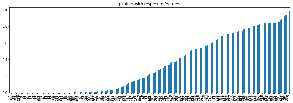
Let's plot the pvalues with respect to the features using the bar plot.

p_values.plot.bar(figsize = (16, 5))
plt.title('pvalues with respect to features')
plt.show()

p_values = p_values[p_values<0.05]

p_values.index

Int64Index([ 40, 182,  86,  22, 101,  51,   2, 127,  49,  91,  30,  27,  61,
             52,  23,  85,  56,  25,  54,  29,  58,  28,  57, 185, 119, 111,
             26,  55,  16,  17,  13,  21,  14,  69,  33, 184,  32,  68, 223,
            178, 109, 224,  36,  34,  15,  18,  44, 168, 221, 198, 199, 100,
            196, 197, 244,  46,  24,  53,  62,  31, 125,  38, 144,  50, 108,
            220, 115, 219, 183,  35,  98, 172,  60,  59, 217, 180,  95,  92,
            166,  72, 105, 209, 202, 211, 186, 212,  70, 110],
           dtype='int64')

X_train_p = X_train_unique[p_values.index]
X_test_p = X_test_unique[p_values.index]

Build the classifiers and compare the performance

Let's build the Random forest classifier and then get the predicted y value.

def run_randomForest(X_train, X_test, y_train, y_test):
    clf = RandomForestClassifier(n_estimators=100, random_state=0, n_jobs = -1)
    clf.fit(X_train, y_train)
    y_pred = clf.predict(X_test)
    print('Accuracy: ', accuracy_score(y_test, y_pred))

Let's calculate the accuracy and training time of trained dataset.

%%time
run_randomForest(X_train_p, X_test_p, y_train, y_test)

Accuracy:  0.953
Wall time: 814 ms

Let's calculate the accuracy and training time of original dataset.

%%time
run_randomForest(X_train, X_test, y_train, y_test)

Accuracy:  0.9585
Wall time: 1.49 s