Feature Selection Based on Univariate ROC_AUC for Classification and MSE for Regression | Machine Learning | KGP talkie
Feature Selection Based on Univariate ROC_AUC for Classification and MSE for Regression
Watch Full Playlist: https://www.youtube.com/playlist?list=PLc2rvfiptPSQYzmDIFuq2PqN2n28ZjxDH
What is ROC_AUC
The Receiver Operator Characteristic (ROC) curve is well-known in evaluating classification performance. Owing to its superiority in dealing with imbalanced and cost-sensitive data, the ROC curve has been exploited as a popular metric to evaluate ML models.
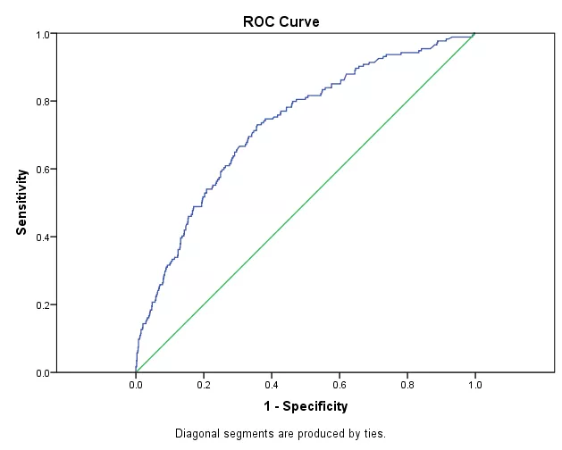
The ROC curve and AUC (area under the ROC curve) have been widely used to determine the classification accuracy in supervised learning.
It is basically used in Binary Classification
Use of ROC_AUC in Classification Problem
Importing required libraries
import numpy as np
import pandas as pd
import matplotlib.pyplot as plt
import seaborn as sns
from sklearn.model_selection import train_test_split
from sklearn.ensemble import RandomForestClassifier
from sklearn.metrics import accuracy_score, roc_auc_score
from sklearn.feature_selection import VarianceThreshold
Download Dataset: https://github.com/laxmimerit/Data-Files-for-Feature-Selection
Let’s read the santander data inti the data variable.
data = pd.read_csv('train.csv', nrows = 20000)
data.head()
| ID | var3 | var15 | imp_ent_var16_ult1 | imp_op_var39_comer_ult1 | imp_op_var39_comer_ult3 | imp_op_var40_comer_ult1 | imp_op_var40_comer_ult3 | imp_op_var40_efect_ult1 | imp_op_var40_efect_ult3 | … | saldo_medio_var33_hace2 | saldo_medio_var33_hace3 | saldo_medio_var33_ult1 | saldo_medio_var33_ult3 | saldo_medio_var44_hace2 | saldo_medio_var44_hace3 | saldo_medio_var44_ult1 | saldo_medio_var44_ult3 | var38 | TARGET | |
|---|---|---|---|---|---|---|---|---|---|---|---|---|---|---|---|---|---|---|---|---|---|
| 0 | 1 | 2 | 23 | 0.0 | 0.0 | 0.0 | 0.0 | 0.0 | 0 | 0 | … | 0.0 | 0.0 | 0.0 | 0.0 | 0.0 | 0.0 | 0.0 | 0.0 | 39205.170000 | 0 |
| 1 | 3 | 2 | 34 | 0.0 | 0.0 | 0.0 | 0.0 | 0.0 | 0 | 0 | … | 0.0 | 0.0 | 0.0 | 0.0 | 0.0 | 0.0 | 0.0 | 0.0 | 49278.030000 | 0 |
| 2 | 4 | 2 | 23 | 0.0 | 0.0 | 0.0 | 0.0 | 0.0 | 0 | 0 | … | 0.0 | 0.0 | 0.0 | 0.0 | 0.0 | 0.0 | 0.0 | 0.0 | 67333.770000 | 0 |
| 3 | 8 | 2 | 37 | 0.0 | 195.0 | 195.0 | 0.0 | 0.0 | 0 | 0 | … | 0.0 | 0.0 | 0.0 | 0.0 | 0.0 | 0.0 | 0.0 | 0.0 | 64007.970000 | 0 |
| 4 | 10 | 2 | 39 | 0.0 | 0.0 | 0.0 | 0.0 | 0.0 | 0 | 0 | … | 0.0 | 0.0 | 0.0 | 0.0 | 0.0 | 0.0 | 0.0 | 0.0 | 117310.979016 | 0 |
5 rows × 371 columns
Here, we will remove the target.
X = data.drop('TARGET', axis = 1)
y = data['TARGET']
X.shape, y.shape
((20000, 370), (20000,))
Let’s split this dataset into train and test datasets using the below code.
Here test_size = 0.2 that means 20% for testing and remaining for training the model.
X_train, X_test, y_train, y_test = train_test_split(X, y, test_size = 0.2, random_state = 0, stratify = y)
Remove Constant, Quasi Constant and Duplicate Features
In this, first we need to create a variance threshold and then fit the model with training set of the data.
#remove constant and quasi constant features
constant_filter = VarianceThreshold(threshold=0.01)
constant_filter.fit(X_train)
X_train_filter = constant_filter.transform(X_train)
X_test_filter = constant_filter.transform(X_test)
X_train_filter.shape, X_test_filter.shape
((16000, 245), (4000, 245))
370-245
125
If two features are exactly same those are called as duplicate features that means these features doesn’t provide any new information and makes our model complex.
Here we have a problem as we did in quasi constant and constant removal sklearn doesn’t have direct library to handle with duplicate features .
So, first we will do transpose the dataset and then python have a method to remove duplicate features.
Let’s transpose the training and testing dataset by using following code.
#remove duplicate features
X_train_T = X_train_filter.T
X_test_T = X_test_filter.T
X_train_T = pd.DataFrame(X_train_T)
X_test_T = pd.DataFrame(X_test_T)
Let’s get the total number of duplicated features .
X_train_T.duplicated().sum()
18
duplicated_features = X_train_T.duplicated()
features_to_keep = [not index for index in duplicated_features]
X_train_unique = X_train_T[features_to_keep].T
X_test_unique = X_test_T[features_to_keep].T
X_train_unique.shape, X_train.shape
((16000, 227), (16000, 370))
Now calculate ROC_AUC Score
NOw, we will calculate roc_auc score for each feature. Let’s have a look at the following code.
roc_auc = []
for feature in X_train_unique.columns:
    clf = RandomForestClassifier(n_estimators=100, random_state=0)
    clf.fit(X_train_unique[feature].to_frame(), y_train)
    y_pred = clf.predict(X_test_unique[feature].to_frame())
    roc_auc.append(roc_auc_score(y_test, y_pred))
print(roc_auc)
[0.5020561820568537, 0.5, 0.5, 0.49986968986187125, 0.501373452866903, 0.49569976544175137, 0.5028068643863192, 0.49986968986187125, 0.5, 0.5, 0.4997393797237425, 0.5017643832812891, 0.49569976544175137, 0.49960906958561374, 0.49895751889497003, 0.49700286682303885, 0.49960906958561374, 0.5021553136956755, 0.4968725566849101, 0.5, 0.5, 0.5, 0.5, 0.5, 0.5, 0.5, 0.5, 0.5, 0.5, 0.5, 0.5, 0.5, 0.5, 0.5, 0.5, 0.5, 0.5, 0.5, 0.5, 0.5, 0.5, 0.5, 0.5, 0.5, 0.5, 0.5, 0.5, 0.5, 0.5, 0.5, 0.5, 0.5, 0.5, 0.5, 0.5, 0.5, 0.5, 0.5, 0.5, 0.5, 0.5, 0.5, 0.5, 0.5, 0.5, 0.5, 0.5, 0.5, 0.5, 0.5, 0.49986968986187125, 0.5, 0.5, 0.5, 0.5, 0.5, 0.5, 0.5, 0.5, 0.5, 0.5, 0.5, 0.5, 0.5, 0.5, 0.5, 0.5, 0.5, 0.5, 0.5, 0.5, 0.5, 0.5, 0.5029371745244479, 0.4959603857180089, 0.5, 0.5048318679438659, 0.4997393797237425, 0.5, 0.5, 0.5, 0.5, 0.5, 0.5, 0.5, 0.49921813917122754, 0.49921813917122754, 0.49824600955181303, 0.5, 0.5, 0.5, 0.4990878290330988, 0.4983763196899418, 0.5, 0.5, 0.5, 0.5, 0.5, 0.5, 0.5, 0.5, 0.5, 0.5, 0.5, 0.5, 0.5, 0.5, 0.5, 0.5, 0.5, 0.5, 0.5, 0.5, 0.5, 0.5, 0.5, 0.5, 0.5025462441100617, 0.4990878290330988, 0.5, 0.5, 0.5, 0.5, 0.5, 0.5, 0.5, 0.5, 0.5, 0.5, 0.5, 0.5, 0.5, 0.5, 0.5, 0.5, 0.5, 0.5, 0.49986968986187125, 0.5, 0.5, 0.5, 0.5, 0.5, 0.5, 0.5, 0.5, 0.5, 0.5, 0.5, 0.5, 0.5, 0.5, 0.5, 0.5, 0.5, 0.5, 0.5, 0.5, 0.5, 0.5, 0.5, 0.5, 0.5, 0.5, 0.5, 0.5, 0.5, 0.4997393797237425, 0.5, 0.5, 0.49986968986187125, 0.4991581805187143, 0.4988272087568413, 0.49674224654678134, 0.4995491109331005, 0.5, 0.5, 0.5022856238338043, 0.5012431427287742, 0.5, 0.5, 0.5, 0.49986968986187125, 0.5, 0.4997393797237425, 0.5, 0.5, 0.5, 0.5, 0.5, 0.5, 0.5, 0.5, 0.5, 0.5, 0.5, 0.5, 0.5, 0.5, 0.5, 0.5, 0.5, 0.5, 0.5, 0.5, 0.5, 0.5076595179963898]
Let’s put these values in the pandas series and sort them into descending order.
roc_values = pd.Series(roc_auc)
roc_values.index = X_train_unique.columns
roc_values.sort_values(ascending =False, inplace = True)
roc_values
244    0.507660
107    0.504832
104    0.502937
6      0.502807
155    0.502546
         ...
18     0.496873
211    0.496742
105    0.495960
12     0.495700
5      0.495700
Length: 227, dtype: float64
The features which are less than or equals to 0.5 won’t provide any information for the classification.
roc_values.plot.bar()
plt.title('roc_auc score with respect to the features')
plt.show()
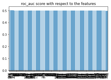
Let’s go ahead and delet the features which have roc_auc score less than 0.5.
sel = roc_values[roc_values>0.5]
sel
244    0.507660
107    0.504832
104    0.502937
6      0.502807
155    0.502546
215    0.502286
17     0.502155
0      0.502056
11     0.501764
4      0.501373
216    0.501243
dtype: float64
Let’s selct new training and testing datasets by using `roc_auc score’.
X_train_roc = X_train_unique[sel.index]
X_test_roc = X_test_unique[sel.index]
Build the Model and compare the performance
We will define a random forest classifier with 100 number of estimators.
def run_randomForest(X_train, X_test, y_train, y_test):
    clf = RandomForestClassifier(n_estimators=100, random_state=0, n_jobs=-1)
    clf.fit(X_train, y_train)
    y_pred = clf.predict(X_test)
    print('Accuracy on test set: ', accuracy_score(y_test, y_pred))
Let’s calculate the accuaracy and training time on test dataset.
%%time
run_randomForest(X_train_roc, X_test_roc, y_train, y_test)
Accuracy on test set:  0.95275
Wall time: 917 ms
X_train_roc.shape
(16000, 11)
Let’s calculate the accuaracy and training time on original test dataset
%%time
run_randomForest(X_train, X_test, y_train, y_test)
Accuracy on test set:  0.9585
Wall time: 1.76 s
Feature Selection using RMSE in Regression
from sklearn.datasets import load_boston
from sklearn.linear_model import LinearRegression
from sklearn.metrics import mean_absolute_error, mean_squared_error, r2_score
boston = load_boston()
print(boston.DESCR)
.. _boston_dataset:

Boston house prices dataset
---------------------------

**Data Set Characteristics:**

    :Number of Instances: 506

    :Number of Attributes: 13 numeric/categorical predictive. Median Value (attribute 14) is usually the target.

    :Attribute Information (in order):
        - CRIM     per capita crime rate by town
        - ZN       proportion of residential land zoned for lots over 25,000 sq.ft.
        - INDUS    proportion of non-retail business acres per town
        - CHAS     Charles River dummy variable (= 1 if tract bounds river; 0 otherwise)
        - NOX      nitric oxides concentration (parts per 10 million)
        - RM       average number of rooms per dwelling
        - AGE      proportion of owner-occupied units built prior to 1940
        - DIS      weighted distances to five Boston employment centres
        - RAD      index of accessibility to radial highways
        - TAX      full-value property-tax rate per $10,000
        - PTRATIO  pupil-teacher ratio by town
        - B        1000(Bk - 0.63)^2 where Bk is the proportion of blacks by town
        - LSTAT    % lower status of the population
        - MEDV     Median value of owner-occupied homes in $1000's

    :Missing Attribute Values: None

    :Creator: Harrison, D. and Rubinfeld, D.L.

This is a copy of UCI ML housing dataset.
https://archive.ics.uci.edu/ml/machine-learning-databases/housing/


This dataset was taken from the StatLib library which is maintained at Carnegie Mellon University.

The Boston house-price data of Harrison, D. and Rubinfeld, D.L. 'Hedonic
prices and the demand for clean air', J. Environ. Economics & Management,
vol.5, 81-102, 1978.   Used in Belsley, Kuh & Welsch, 'Regression diagnostics
...', Wiley, 1980.   N.B. Various transformations are used in the table on
pages 244-261 of the latter.

The Boston house-price data has been used in many machine learning papers that address regression
problems.

.. topic:: References

   - Belsley, Kuh & Welsch, 'Regression diagnostics: Identifying Influential Data and Sources of Collinearity', Wiley, 1980. 244-261.
   - Quinlan,R. (1993). Combining Instance-Based and Model-Based Learning. In Proceedings on the Tenth International Conference of Machine Learning, 236-243, University of Massachusetts, Amherst. Morgan Kaufmann.
X = pd.DataFrame(boston.data, columns=boston.feature_names)
X.head()
| CRIM | ZN | INDUS | CHAS | NOX | RM | AGE | DIS | RAD | TAX | PTRATIO | B | LSTAT | |
|---|---|---|---|---|---|---|---|---|---|---|---|---|---|
| 0 | 0.00632 | 18.0 | 2.31 | 0.0 | 0.538 | 6.575 | 65.2 | 4.0900 | 1.0 | 296.0 | 15.3 | 396.90 | 4.98 |
| 1 | 0.02731 | 0.0 | 7.07 | 0.0 | 0.469 | 6.421 | 78.9 | 4.9671 | 2.0 | 242.0 | 17.8 | 396.90 | 9.14 |
| 2 | 0.02729 | 0.0 | 7.07 | 0.0 | 0.469 | 7.185 | 61.1 | 4.9671 | 2.0 | 242.0 | 17.8 | 392.83 | 4.03 |
| 3 | 0.03237 | 0.0 | 2.18 | 0.0 | 0.458 | 6.998 | 45.8 | 6.0622 | 3.0 | 222.0 | 18.7 | 394.63 | 2.94 |
| 4 | 0.06905 | 0.0 | 2.18 | 0.0 | 0.458 | 7.147 | 54.2 | 6.0622 | 3.0 | 222.0 | 18.7 | 396.90 | 5.33 |
y = boston.target
X_train, X_test, y_train, y_test = train_test_split(X, y, test_size = 0.2, random_state = 0)
Let’s calculate the mean square error(mse) between testing and predicting values of y
mse = []
for feature in X_train.columns:
    clf = LinearRegression()
    clf.fit(X_train[feature].to_frame(), y_train)
    y_pred = clf.predict(X_test[feature].to_frame())
    mse.append(mean_squared_error(y_test, y_pred))
mse
[76.38674157646072,
 84.66034377707905,
 77.02905244667242,
 79.36120219345942,
 76.95375968209433,
 46.907351627395315,
 80.3915476111525,
 82.61874125667718,
 82.46499985731933,
 78.30831374720843,
 81.79497121208001,
 77.75285601192718,
 46.33630536002592]
Let’s sort the mean square error values in descending order. Let’s have a look at the following code.
mse = pd.Series(mse, index = X_train.columns)
mse.sort_values(ascending=False, inplace = True)
mse
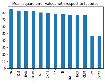
ZN         84.660344
DIS        82.618741
RAD        82.465000
PTRATIO    81.794971
AGE        80.391548
CHAS       79.361202
TAX        78.308314
B          77.752856
INDUS      77.029052
NOX        76.953760
CRIM       76.386742
RM         46.907352
LSTAT      46.336305
dtype: float64
Let’s observe the mean square error values with respect to features from the following bar plot.
mse.plot.bar()
plt.title('Mean square error values with respect to features')
plt.show()
Let’s create testing and training datasets based on only two features.
X_train_2 = X_train[['RM', 'LSTAT']]
X_test_2 = X_test[['RM', 'LSTAT']]
Now, we will calculate the performance with the selected features.
%%time
model = LinearRegression()
model.fit(X_train_2, y_train)
y_pred = model.predict(X_test_2)
print('r2_score: ', r2_score(y_test, y_pred))
print('rmse: ', np.sqrt(mean_squared_error(y_test, y_pred)))
print('sd of house price: ', np.std(y))
r2_score:  0.5409084827186417
rmse:  6.114172522817782
sd of house price:  9.188011545278203
Wall time: 3 ms
Now, we will calculate the performance with the original features.
%%time
model = LinearRegression()
model.fit(X_train, y_train)
y_pred = model.predict(X_test)
print('r2_score: ', r2_score(y_test, y_pred))
print('rmse: ', np.sqrt(mean_squared_error(y_test, y_pred)))
print('sd of house price: ', np.std(y))
r2_score:  0.5892223849182507
rmse:  5.783509315085135
sd of house price:  9.188011545278203
Wall time: 4 ms
0 Comments