
When you train a machine learning model on too many features, it can memorize patterns in the training data that do not generalize to new data — a problem called overfitting. One of the most effective ways to fight overfitting is regularization — adding a penalty to the model that discourages large coefficients.
What makes regularization especially useful for feature selection is that the L1 variant (called Lasso) can push the coefficients of unimportant features all the way to zero. A feature with a zero coefficient contributes nothing to the prediction, so Lasso effectively removes it from the model automatically. This makes Lasso an embedded feature selection method — the selection happens as part of the training process, not as a separate preprocessing step.
In this tutorial you will apply Lasso and Ridge regularization to the Titanic survival dataset. You will use SelectFromModel from Scikit-Learn to extract the features Lasso considers important, then compare model accuracy against a Ridge classifier tuned with cross-validation.
Prerequisites: Python 3.x, Scikit-learn, Pandas, NumPy, Seaborn, Matplotlib.
What is Regularization?
Every supervised model tries to minimize a loss function — for linear models that is typically the Residual Sum of Squares (RSS), which measures how far the model's predictions are from the true labels. The problem is that minimizing RSS alone can produce very large coefficients that fit training noise perfectly but fail on unseen data.
Regularization fixes this by adding an extra term to the loss function that penalizes large coefficients. The model must now find a balance: reduce prediction error while also keeping coefficients small.
There are two common penalty types:
- L1 Regularization (Lasso) — penalizes the sum of the absolute values of the coefficients. This can shrink some coefficients to exactly zero, removing their features from the model entirely.
- L2 Regularization (Ridge) — penalizes the sum of the squared values of the coefficients. This shrinks all coefficients toward zero but rarely reaches exactly zero, so all features remain in the model with reduced influence.
- Elastic Net — combines both L1 and L2 penalties, giving you the benefits of each.
Bias, Variance, and Model Complexity
To understand why regularization works, you need to understand bias and variance — the two main sources of prediction error you can actually control.
- Bias error measures how far the model's average predictions are from the true values. A high-bias model is too simple and consistently wrong in the same direction (underfitting).
- Variance measures how much the model's predictions change when trained on different samples of the data. A high-variance model is too complex and fits training noise (overfitting).
The diagram below shows how these two errors behave as model complexity increases:
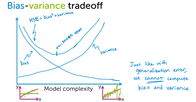
As complexity rises, bias falls but variance climbs. The total error (MSE = bias² + variance) has a sweet spot — the optimal model complexity where the combined error is lowest. Regularization is a direct tool for controlling this tradeoff: a stronger penalty reduces variance at the cost of a small increase in bias.
Lasso (L1) Regularization
The Lasso loss function adds the L1 norm of the weight vector to the RSS:
Where:
- — the true label for the -th training sample
- — the model's regression coefficients (one per feature)
- — the feature values for sample
- — the regularization strength; higher values impose a stronger penalty
- — the L1 norm, i.e., the sum of absolute coefficient values
Because the L1 penalty creates sharp corners in the constraint geometry, the optimizer frequently lands on solutions where some coefficients are exactly zero. The plot below shows Lasso coefficient paths as the regularization strength increases — several features are driven to zero well before others:
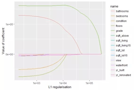
Features whose coefficients reach zero can be dropped from the model entirely. This is the core mechanism behind Lasso as a feature selector.
Choosing the Regularization Strength λ
The value of determines how aggressively the model penalizes large coefficients. Too small a gives you almost no regularization; too large a forces all coefficients toward zero and produces a useless model. The plot below shows how the test error (RMSE) evolves as increases:
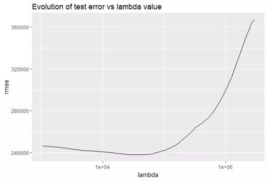
The curve has a clear minimum — the optimal sits at the bottom.
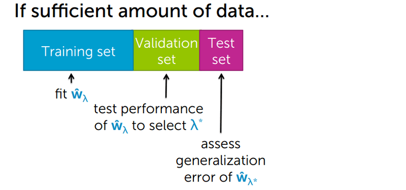
The standard method for finding this value is to split your data into three parts:
- Training set — fit the model and learn the coefficients for a given .
- Validation set — measure performance to pick the best without touching the test set.
- Test set — assess the final generalization error once after selecting .
The diagram below illustrates this three-way split and how each set is used:
Ridge (L2) Regularization
Ridge regularization uses the squared L2 norm of the weight vector instead of the absolute values:
Where:
- — residual sum of squares, the standard least-squares prediction error
- — regularization strength; controls the balance between fit quality and coefficient size
- — the squared L2 norm, i.e., the sum of squared coefficient values
The diagram below summarizes the practical effect of in Ridge:
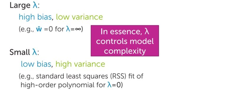
A large pushes all coefficients close to zero (high bias, low variance). A small approaches standard least-squares regression (low bias, high variance). Because the L2 penalty uses squares rather than absolute values, it never forces a coefficient to exactly zero — it only shrinks them progressively. The Ridge coefficient path confirms this:
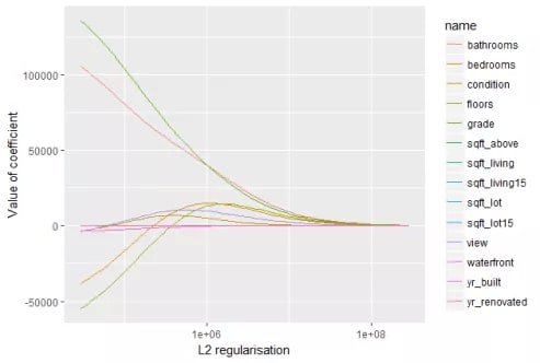
Compare this to the Lasso plot: Ridge coefficients decrease smoothly but remain non-zero, while Lasso coefficients hit zero abruptly. This is why Lasso selects features and Ridge does not.
Lasso Feature Selection on Titanic
Now you will apply everything above to a real classification problem. The goal is to predict whether a Titanic passenger survived using a subset of features selected by Lasso regularization.
Load and Clean the Data
Import all required libraries in one block:
import numpy as np
import pandas as pd
import seaborn as sns
import matplotlib.pyplot as plt
%matplotlib inlinefrom sklearn.model_selection import train_test_split
from sklearn.ensemble import RandomForestClassifier
from sklearn.linear_model import Lasso, LogisticRegression
from sklearn.feature_selection import SelectFromModel
from sklearn.preprocessing import StandardScaler
from sklearn.metrics import accuracy_scoreLoad the Titanic dataset and check for missing values:
titanic = sns.load_dataset('titanic')
titanic.isnull().sum()survived 0
pclass 0
sex 0
age 177
sibsp 0
parch 0
fare 0
embarked 2
class 0
who 0
adult_male 0
deck 688
embark_town 2
alive 0
alone 0
dtype: int64The age column has 177 missing values and deck has 688 — too many to impute reliably. Drop them both:
titanic.drop(labels = ['age', 'deck'], axis = 1, inplace = True)Drop the remaining rows with any missing values and confirm the dataset is clean:
titanic = titanic.dropna()
titanic.isnull().sum()survived 0
pclass 0
sex 0
sibsp 0
parch 0
fare 0
embarked 0
class 0
who 0
adult_male 0
embark_town 0
alive 0
alone 0
dtype: int64Inspect the first few rows to understand the structure:
titanic.head()| survived | pclass | sex | sibsp | parch | fare | embarked | class | who | adult_male | embark_town | alive | alone | |
|---|---|---|---|---|---|---|---|---|---|---|---|---|---|
| 0 | 0 | 3 | male | 1 | 0 | 7.2500 | S | Third | man | True | Southampton | no | False |
| 1 | 1 | 1 | female | 1 | 0 | 71.2833 | C | First | woman | False | Cherbourg | yes | False |
| 2 | 1 | 3 | female | 0 | 0 | 7.9250 | S | Third | woman | False | Southampton | yes | True |
| 3 | 1 | 1 | female | 1 | 0 | 53.1000 | S | First | woman | False | Southampton | yes | False |
| 4 | 0 | 3 | male | 0 | 0 | 8.0500 | S | Third | man | True | Southampton | no | True |
Prepare Features
Select the seven features you will use for classification:
data = titanic[['pclass', 'sex', 'sibsp', 'parch', 'embarked', 'who', 'alone']].copy()data.head()| pclass | sex | sibsp | parch | embarked | who | alone | |
|---|---|---|---|---|---|---|---|
| 0 | 3 | male | 1 | 0 | S | man | False |
| 1 | 1 | female | 1 | 0 | C | woman | False |
| 2 | 3 | female | 0 | 0 | S | woman | True |
| 3 | 1 | female | 1 | 0 | S | woman | False |
| 4 | 3 | male | 0 | 0 | S | man | True |
Encode the categorical columns as integers so they can be passed to a linear model:
sex = {'male': 0, 'female': 1}
data['sex'] = data['sex'].map(sex)                       ports = {'S': 0, 'C': 1, 'Q': 2}
data['embarked'] = data['embarked'].map(ports)             who = {'man': 0, 'woman': 1, 'child': 2}
data['who'] = data['who'].map(who)                       alone = {True: 1, False: 0}
data['alone'] = data['alone'].map(alone)
Assign features to X and the target to y, then split into training and test sets:
X = data.copy()
y = titanic['survived']
x.head()| No. | pclass | sex | sibsp | parch | embarked | who | alone |
|---|---|---|---|---|---|---|---|
| 0 | 3 | 0 | 1 | 0 | 0 | 0 | 0 |
| 1 | 1 | 1 | 1 | 0 | 1 | 1 | 0 |
| 2 | 3 | 1 | 0 | 0 | 0 | 1 | 1 |
| 3 | 1 | 1 | 1 | 0 | 0 | 1 | 0 |
| 4 | 3 | 0 | 0 | 0 | 0 | 0 | 1 |
X_train, X_test, y_train, y_test = train_test_split(X, y, test_size = 0.33, random_state = 42)Select Features with SelectFromModel
SelectFromModel is a meta-transformer — it wraps any estimator that produces coefficients or feature importances and uses those values to select the most important features. Here you wrap a LogisticRegression with L1 penalty (penalty='l1') and a small C value. C is the inverse of the regularization strength — a small C means strong regularization, which forces more coefficients to zero:
sel = SelectFromModel(LogisticRegression(C = 0.05, penalty = 'l1', solver = 'liblinear'))
sel.fit(X_train, y_train)SelectFromModel(estimator=LogisticRegression(C=0.05, penalty='l1', solver='liblinear'))get_support() returns a boolean mask showing which features were kept (True) and which were eliminated (False):
sel.get_support()array([ True, True, True, False, False, True, False])Four features were selected. Retrieve their names:
features = X_train.columns[sel.get_support()]
featuresIndex(['pclass', 'sex', 'sibsp', 'who'], dtype='object')Lasso kept pclass, sex, sibsp, and who — the features most correlated with survival. Apply the transformation to produce reduced training and test sets:
X_train_l1 = sel.transform(X_train)
X_test_l1 = sel.transform(X_test)
X_train_l1.shape, X_test_l1.shape((595, 4), (294, 4))The training set now has 4 columns instead of 7, and the test set matches.
Build and Compare Random Forest Models
Define a helper function that trains a RandomForestClassifier and prints the accuracy:
def run_randomForest(X_train, X_test, y_train, y_test):
    clf = RandomForestClassifier(n_estimators=100, random_state=0, n_jobs = -1)
    clf.fit(X_train, y_train)
    y_pred = clf.predict(X_test)
    print('Accuracy: ', accuracy_score(y_test, y_pred))
Train on the Lasso-selected features (4 columns):
%%time
run_randomForest(X_train_l1, X_test_l1, y_train, y_test)Accuracy: 0.826530612244898
Wall time: 517 msTrain on all 7 original features for comparison:
%%time
run_randomForest(X_train, X_test, y_train, y_test)Accuracy: 0.8163265306122449
Wall time: 169 msThe Lasso-selected model achieves 82.7 % accuracy versus 81.6 % for the full feature set — removing the three weakest features actually improved performance slightly, showing that those features were adding noise rather than signal.
Ridge Regression for Classification
Ridge regularization is available for classification through RidgeClassifier. Import it:
from sklearn.linear_model import RidgeClassifierFit a Ridge classifier with a fixed alpha of 300 (alpha is equivalent to in the formula — a larger value means stronger regularization):
rr = RidgeClassifier(alpha=300)
rr.fit(X_train, y_train)               RidgeClassifier(alpha=300)
Check the accuracy on the test set:
rr.score(X_test, y_test)0.8231292517006803Inspect the coefficients — because Ridge uses L2 regularization, none of them are exactly zero:
rr.coef_array([[-0.20537487, 0.24017869, -0.07964489, -0.00072071, 0.05154718, 0.26474716, -0.07454003]])All seven features remain in the model, but the smaller coefficients reveal the less influential features (parch at −0.00072 is nearly irrelevant).
Tune Alpha with Cross-Validation
Instead of guessing alpha, use RidgeClassifierCV to find the best value automatically. It performs Generalized Cross-Validation (GCV) — an efficient approximation of Leave-One-Out cross-validation — across every alpha you specify:
from sklearn.linear_model import RidgeClassifierCVrr = RidgeClassifierCV(alphas=[10, 20, 50, 100, 200, 300], cv = 10 )
rr.fit(X_train, y_train) RidgeClassifierCV(alphas=array([ 10, 20, 50, 100, 200, 300]), cv=10)Evaluate on the test set:
rr.score(X_test, y_test)0.8197278911564626Read the coefficients the cross-validated model learned:
rr.coef_array([[-0.23422431, 0.29215915, -0.09681069, -0.01263653, 0.05860246, 0.31323408, -0.09073738]])Check which alpha was selected as the best:
rr.alpha_200Confirm the full list of candidates that were evaluated:
rr.alphasarray([ 10, 20, 50, 100, 200, 300])RidgeClassifierCV selected alpha=200 as the best regularization strength across 10-fold cross-validation, achieving approximately 82 % accuracy.
Conclusion
In this tutorial you used Lasso (L1) and Ridge (L2) regularization as embedded feature selection methods on the Titanic dataset. Lasso's SelectFromModel pipeline automatically eliminated three of seven features, and the resulting Random Forest model scored 82.7 % — slightly better than using all features. The Ridge classifier with cross-validated alpha selection achieved 82 % using all features with shrunk coefficients.
Key takeaways:
- Lasso (L1) forces some coefficients to exactly zero, making it a true feature selector; features with zero coefficients can be safely dropped.
- Ridge (L2) shrinks all coefficients toward zero but never eliminates any feature; it reveals relative importance rather than performing hard selection.
SelectFromModelwraps any coefficient-based estimator and turns it into a feature selection transformer compatible with any Scikit-Learn pipeline.RidgeClassifierCVautomates regularization strength tuning via cross-validation, removing the need to guess alpha manually.- Removing weak features with Lasso can improve model accuracy by reducing noise, even when the number of features is small.
Next steps:
- Explore how raw regression coefficients compare to regularized ones in Use of Linear and Logistic Regression Coefficients with Lasso and Ridge for Feature Selection.
- Apply a model-agnostic wrapper approach in Recursive Feature Elimination (RFE) using tree-based and gradient-based estimators.
- Start from first principles with statistical filters in Feature Selection with Filter Methods to see how constant, quasi-constant, and duplicate features are removed before modeling.

