
When you train a regression model, each feature gets a coefficient — a number that tells you how strongly that feature influences the prediction. Features with large coefficients matter a lot; features with coefficients near zero contribute almost nothing. Regularization — adding a penalty to the model's loss function — forces these coefficients to shrink, and with the right type of regularization you can push the weakest ones all the way to zero, automatically eliminating those features.
This tutorial shows you how to apply that idea in practice. You will use the Titanic dataset to select features with two regularized models: a plain Linear Regression (unregularized, as a baseline), a Logistic Regression with L1 (Lasso) penalty, and a Logistic Regression with L2 (Ridge) penalty. For each approach you will extract the selected features with SelectFromModel, then measure accuracy using a Random Forest classifier on the pruned feature set.
Prerequisites: Python 3.x, scikit-learn, Pandas, NumPy, Seaborn.
Linear Regression and Coefficient-Based Feature Importance
Linear regression predicts a continuous target variable as a weighted sum of input features. The weight assigned to each feature is its coefficient, and the magnitude of that coefficient tells you how important the feature is.
The model takes this form:
Where:
- — the target value for observation
- — the intercept (the predicted value when all features are zero)
- — the regression coefficient (how much changes for a one-unit increase in )
- — the predictor (input) feature for observation
- — the random error term (noise not captured by the model)
Assumptions of Linear Regression
For coefficient magnitudes to reliably rank feature importance, the model's core assumptions should hold:
- There is a linear relationship between each feature and the target .
- Each feature should be roughly normally (Gaussian) distributed.
- Features should not be highly correlated with each other (multicollinearity can distort coefficients).
- Features should be on the same scale — if one feature is measured in thousands and another in fractions, their raw coefficients are not directly comparable.
Lasso (L1) and Ridge (L2) Regularization
Without regularization, a linear model freely assigns large coefficients, which can lead to overfitting — the model memorizes the training data but performs poorly on new data. Regularization adds a penalty term to the loss function that discourages large coefficients, keeping the model simpler and more general.
There are two main forms:
- L1 regularization (Lasso): Penalizes the sum of the absolute values of the coefficients. This penalty can shrink weak coefficients all the way to exactly zero, effectively removing those features from the model. Lasso is therefore a built-in feature selection method.
- L2 regularization (Ridge): Penalizes the sum of the squared values of the coefficients. This shrinks all coefficients toward zero but rarely reaches exactly zero, so all features are retained. You can still use coefficient magnitude to rank importance.
- Elastic Net (L1 + L2 combined): A hybrid that blends both penalties, balancing sparsity and stability.
Before diving into the code, it is worth understanding the bias-variance tradeoff that regularization manages. The diagram below illustrates how total prediction error decomposes into bias and variance as model complexity changes:
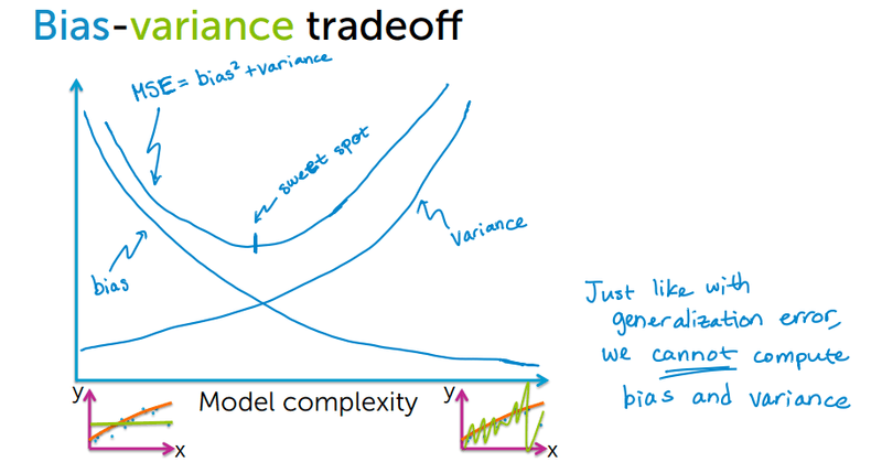
Increasing model complexity reduces bias but increases variance. Regularization lets you tune this tradeoff by controlling the strength of the penalty with a parameter .
Lasso (L1) Regularization
The Lasso loss function is the standard residual sum of squares plus the L1 penalty:

Where:
- — residual sum of squares: the total squared difference between actual and predicted values
- — regularization strength; a larger applies a heavier penalty
- — the regression coefficient for feature
- — the total number of features
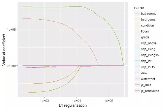
Because the L1 penalty uses absolute values, its gradient has a constant magnitude, which can push coefficients to exactly zero. The chart below shows how Lasso coefficient paths evolve as the L1 regularization strength increases — most features are driven to zero at high penalty values:
Choosing the Regularization Strength λ
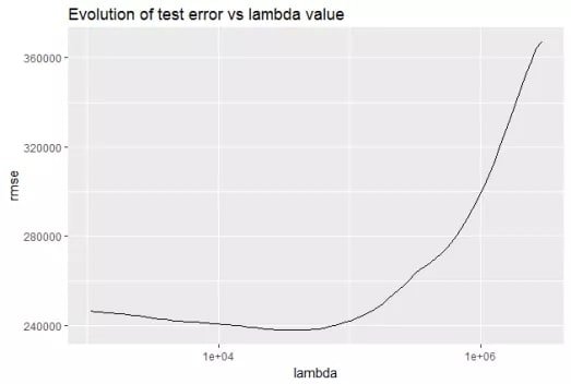
The choice of controls how aggressively the model penalizes complexity. You can observe its effect by plotting test error against different values of : error first falls as the model becomes less overfit, then rises again once the model is too constrained:
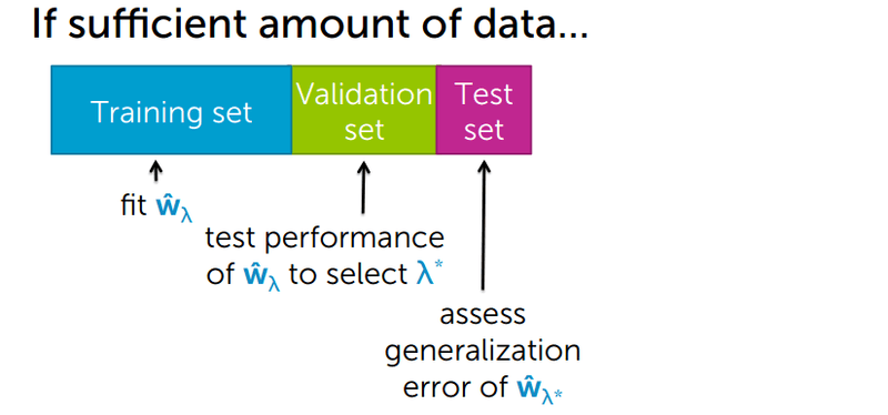
To find the optimal , split your data into three parts:
- Training set: Fit the model and learn the regression coefficients with regularization applied.
- Validation set: Evaluate model performance to choose the best . If accuracy is insufficient, adjust and retrain.
- Test set: Final evaluation of generalization error using the selected on the validation set.
The diagram below shows which role each split plays:
Ridge Regularization (L2)
Ridge regression adds a penalty equal to the sum of the squared coefficient values:
Where:
- — residual sum of squares
- — regularization strength (tuning parameter)
- — the regression coefficient for feature
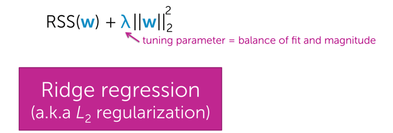
The L2 squared penalty has a smooth gradient that never reaches exactly zero, so Ridge keeps all features in the model but makes their coefficients small. The diagram below names this quantity and highlights the role of as a balance between fit quality and coefficient magnitude:
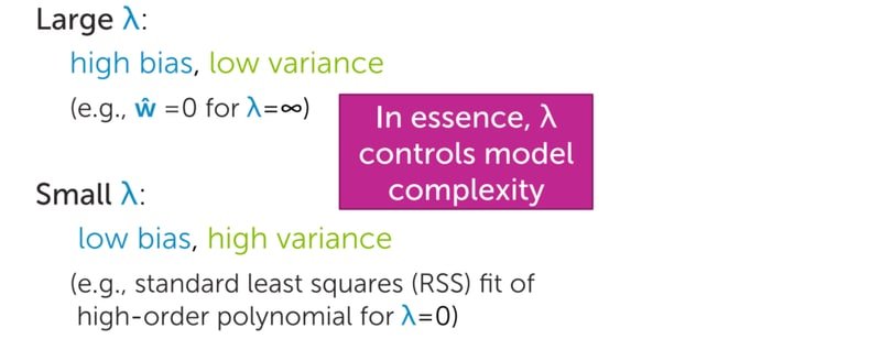
The effect of on model behavior is straightforward: a large produces high bias and low variance (all coefficients near zero); a small produces low bias and high variance (coefficients grow freely):
As you increase L2 regularization, all coefficients shrink smoothly toward zero without crossing it. The chart below illustrates this gradual shrinkage across features:
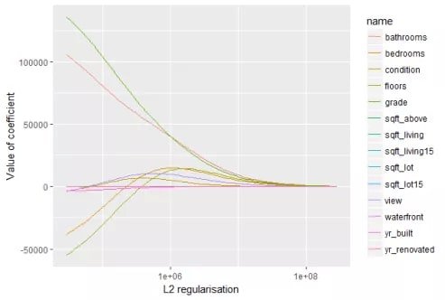
The L2 regularization forces parameters to stay relatively small. The bigger the penalty, the smaller and more stable the coefficients become — but no feature is ever fully eliminated.
Difference Between L1 and L2 Regularization
| L1 Regularization | L2 Regularization |
|---|---|
| It penalizes sum of absolute value of weights | It regularization penalizes sum of square weights |
| It has a sparse solution | It has a non sparse solution |
| It has multiple solutions | It has one solution |
| It has built in feature selection | It has no feature selection |
| It is robust to outliers | It is not robust to outliers |
| It generates model that are simple and interpretable but cannot learn complex patterns | It gives better prediction when output variable is a function of all input features |
Feature Selection on the Titanic Dataset
With the theory in place, you can now apply both regularization methods to a real dataset. The goal is to predict Titanic passenger survival using a subset of features selected by regularized regression.
Start by importing all the libraries you need:
import numpy as np
import pandas as pd
import seaborn as sns
import matplotlib.pyplot as plt
%matplotlib inlinefrom sklearn.model_selection import train_test_split
from sklearn.ensemble import RandomForestClassifier
from sklearn.feature_selection import SelectKBest, SelectPercentile
from sklearn.metrics import accuracy_scorefrom sklearn.linear_model import LinearRegression, LogisticRegression
from sklearn.feature_selection import SelectFromModelLoad the Titanic dataset from Seaborn and inspect the first few rows:
titanic = sns.load_dataset('titanic')
titanic.head()| survived | pclass | sex | age | sibsp | parch | fare | embarked | class | who | adult_male | deck | embark_town | alive | alone | |
|---|---|---|---|---|---|---|---|---|---|---|---|---|---|---|---|
| 0 | 0 | 3 | male | 22.0 | 1 | 0 | 7.2500 | S | Third | man | True | NaN | Southampton | no | False |
| 1 | 1 | 1 | female | 38.0 | 1 | 0 | 71.2833 | C | First | woman | False | C | Cherbourg | yes | False |
| 2 | 1 | 3 | female | 26.0 | 0 | 0 | 7.9250 | S | Third | woman | False | NaN | Southampton | yes | True |
| 3 | 1 | 1 | female | 35.0 | 1 | 0 | 53.1000 | S | First | woman | False | C | Southampton | yes | False |
| 4 | 0 | 3 | male | 35.0 | 0 | 0 | 8.0500 | S | Third | man | True | NaN | Southampton | no | True |
Check how many missing values exist in each column:
titanic.isnull().sum()survived 0
pclass 0
sex 0
age 177
sibsp 0
parch 0
fare 0
embarked 2
class 0
who 0
adult_male 0
deck 688
embark_town 2
alive 0
alone 0
dtype: int64The age column has 177 missing values and deck has 688 — too many to impute reliably. Drop both columns and then remove any remaining rows with nulls:
titanic.drop(labels = ['age', 'deck'], axis = 1, inplace = True)
titanic = titanic.dropna()
titanic.isnull().sum()survived 0
pclass 0
sex 0
sibsp 0
parch 0
fare 0
embarked 0
class 0
who 0
adult_male 0
embark_town 0
alive 0
alone 0
dtype: int64Select the seven features you will use for prediction:
data = titanic[['pclass', 'sex', 'sibsp', 'parch', 'embarked', 'who', 'alone']].copy()
data.head()| pclass | sex | sibsp | parch | embarked | who | alone | |
|---|---|---|---|---|---|---|---|
| 0 | 3 | male | 1 | 0 | S | man | False |
| 1 | 1 | female | 1 | 0 | C | woman | False |
| 2 | 3 | female | 0 | 0 | S | woman | True |
| 3 | 1 | female | 1 | 0 | S | woman | False |
| 4 | 3 | male | 0 | 0 | S | man | True |
Confirm there are no missing values in the feature set:
data.isnull().sum()pclass 0
sex 0
sibsp 0
parch 0
embarked 0
who 0
alone 0
dtype: int64The categorical columns must be encoded as integers before fitting a regression model. Encode sex, embarked, who, and alone:
sex = {'male': 0, 'female': 1}
data['sex'] = data['sex'].map(sex)
data.head()| pclass | sex | sibsp | parch | embarked | who | alone | |
|---|---|---|---|---|---|---|---|
| 0 | 3 | 0 | 1 | 0 | S | man | False |
| 1 | 1 | 1 | 1 | 0 | C | woman | False |
| 2 | 3 | 1 | 0 | 0 | S | woman | True |
| 3 | 1 | 1 | 1 | 0 | S | woman | False |
| 4 | 3 | 0 | 0 | 0 | S | man | True |
ports = {'S': 0, 'C': 1, 'Q': 2}
data['embarked'] = data['embarked'].map(ports)
who = {'man': 0, 'woman': 1, 'child': 2}
data['who'] = data['who'].map(who)
alone = {True: 1, False: 0}
data['alone'] = data['alone'].map(alone)
data.head()| pclass | sex | sibsp | parch | embarked | who | alone | |
|---|---|---|---|---|---|---|---|
| 0 | 3 | 0 | 1 | 0 | 0 | 0 | 0 |
| 1 | 1 | 1 | 1 | 0 | 1 | 1 | 0 |
| 2 | 3 | 1 | 0 | 0 | 0 | 1 | 1 |
| 3 | 1 | 1 | 1 | 0 | 0 | 1 | 0 |
| 4 | 3 | 0 | 0 | 0 | 0 | 0 | 1 |
Separate features from the target label and check the resulting shapes:
X = data.copy()
y = titanic['survived']
X.shape, y.shape((889, 7), (889,))Split the data into training (70%) and test (30%) sets:
X_train, X_test, y_train, y_test = train_test_split(X, y, test_size = 0.3, random_state = 43)Estimating Linear Regression Coefficients
SelectFromModel wraps any estimator and keeps only the features whose absolute coefficient exceeds a threshold (the mean by default). Wrap a plain LinearRegression to use its coefficients as importance scores:
sel = SelectFromModel(LinearRegression())Fit the selector on the training data:
sel.fit(X_train, y_train)
SelectFromModel(estimator=LinearRegression(copy_X=True, fit_intercept=True, n_jobs=None,
         normalize=False),
        max_features=None, norm_order=1, prefit=False, threshold=None)
Call get_support() to see which of the seven features were selected (True) and which were dropped:
sel.get_support()array([ True, True, False, False, False, True, False])Three features passed the threshold. Inspect the raw coefficients to understand why:
sel.estimator_.coef_array([-0.13750402, 0.26606466, -0.07470416, -0.0668525 , 0.04793674,
0.23857799, -0.12929595])The mean absolute coefficient is the default threshold for SelectFromModel. Calculate it to confirm:
mean = np.mean(np.abs(sel.estimator_.coef_))
mean0.13727657291370804Features with an absolute coefficient above this mean are kept. Compare each coefficient's absolute value against that threshold:
np.abs(sel.estimator_.coef_)array([0.13750402, 0.26606466, 0.07470416, 0.0668525 , 0.04793674,
0.23857799, 0.12929595])The three features above the threshold of 0.137 are pclass, sex, and who. Retrieve their names directly:
features = X_train.columns[sel.get_support()]
featuresIndex(['pclass', 'sex', 'who'], dtype='object')Apply the selector to reduce both training and test sets to the three chosen features:
X_train_reg = sel.transform(X_train)
X_test_reg = sel.transform(X_test)
X_test_reg.shape(267, 3)Define a helper function that trains a RandomForestClassifier and prints accuracy and wall time — you will reuse this for every feature set:
def run_randomForest(X_train, X_test, y_train, y_test):
    clf = RandomForestClassifier(n_estimators=100, random_state=0, n_jobs=-1)
    clf = clf.fit(X_train, y_train)
    y_pred = clf.predict(X_test)
    print('Accuracy: ', accuracy_score(y_test, y_pred))
Benchmark accuracy on the three-feature subset selected by Linear Regression:
%%time
run_randomForest(X_train_reg, X_test_reg, y_train, y_test)Accuracy: 0.8239700374531835
Wall time: 250 msCompare against accuracy on the full seven-feature set to verify no information was lost:
%%time
run_randomForest(X_train, X_test, y_train, y_test)Accuracy: 0.8239700374531835
Wall time: 252 msThe accuracy is identical (82.4%) on both the pruned and full feature sets. Confirm the original training size:
X_train.shape(622, 7)The three selected features carry all the predictive signal — the remaining four add no value.
Logistic Regression Coefficients with L1 Regularization
Now apply Lasso regularization via LogisticRegression with penalty='l1'. The C parameter is the inverse of regularization strength — a smaller C applies a stronger penalty and drives more coefficients to zero:
sel = SelectFromModel(LogisticRegression(penalty = 'l1', C = 0.05, solver = 'liblinear'))
sel.fit(X_train, y_train)
sel.get_support()array([ True, True, True, False, False, True, False])Lasso selected four features this time. Inspect the raw coefficients — notice that two of them are exactly zero:
sel.estimator_.coef_array([[-0.54045394, 0.78039608, -0.14081954, 0., 0. ,0.94106713, 0.]])parch, embarked, and alone received zero coefficients and were dropped. Transform the feature sets:
X_train_l1 = sel.transform(X_train)
X_test_l1 = sel.transform(X_test)
Measure accuracy on the Lasso-selected feature subset:
%%time
run_randomForest(X_train_l1, X_test_l1, y_train, y_test)Accuracy: 0.8277153558052435
Wall time: 251 msThe L1-selected model reaches 82.8% accuracy — a marginal improvement over the unregularized Linear Regression selection, using one additional feature (sibsp).
Feature Selection with L2 Regularization
Apply Ridge regularization via LogisticRegression with penalty='l2' and the same C=0.05:
sel = SelectFromModel(LogisticRegression(penalty = 'l2', C = 0.05, solver = 'liblinear'))
sel.fit(X_train, y_train)
sel.get_support()array([ True, True, False, False, False, True, False])Ridge selected the same three features as the unregularized baseline. Check the coefficients — unlike Lasso, none reach exactly zero:
sel.estimator_.coef_array([[-0.55749685, 0.85692344, -0.30436065, -0.11841967, 0.2435823 ,
1.00124155, -0.29875898]])All seven features have non-zero coefficients, but only three exceed the mean absolute threshold. Apply the transform:
X_train_l1 = sel.transform(X_train)
X_test_l1 = sel.transform(X_test)
Benchmark accuracy on the Ridge-selected feature subset:
%%time
run_randomForest(X_train_l1, X_test_l1, y_train, y_test)Accuracy: 0.8239700374531835
Wall time: 250 msThe Ridge-selected model achieves the same 82.4% accuracy as the full feature set, confirming that the three features (pclass, sex, who) capture all the relevant signal in this dataset.
Conclusion
In this tutorial you applied Linear Regression, Lasso (L1), and Ridge (L2) regularized Logistic Regression to the Titanic dataset using scikit-learn's SelectFromModel. All three methods converged on pclass, sex, and who as the most important features, achieving 82.4% accuracy — identical to training on all seven features. The Lasso model added sibsp and achieved a marginal 82.8% accuracy by explicitly zeroing out the weakest coefficients.
Key takeaways:
- Regression coefficients are a direct measure of feature importance — features with larger absolute coefficients contribute more to the prediction.
- L1 (Lasso) regularization can push coefficients to exactly zero, performing automatic feature elimination without any manual threshold tuning.
- L2 (Ridge) regularization shrinks all coefficients without eliminating any — it is better used for ranking features than for hard selection.
SelectFromModelprovides a clean, pipeline-compatible API to extract the features that pass a coefficient threshold from any regularized estimator.- Matching accuracy on a pruned subset confirms the removed features were genuinely uninformative — not just low-coefficient due to scaling.
Next steps:
- Explore Lasso and Ridge for Classification Feature Selection for a deeper look at regularization in classification settings.
- Compare embedded selection with wrapper-based approaches in Recursive Feature Elimination to see how tree-based estimators rank features differently.
- Apply forward and backward search strategies in Step Forward and Step Backward Feature Selection to systematically test every feature combination.

