
Random Forest is one of the most practical and widely-used machine learning algorithms available today. It powers recommendation engines, fraud detection systems, and medical diagnosis tools — anywhere a single model would be too fragile, a forest of models provides the robustness you need.
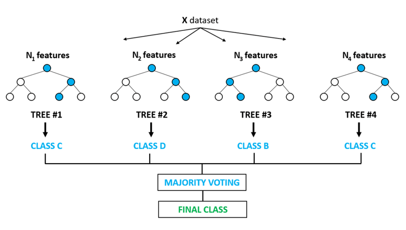
A Random Forest is an ensemble method that builds many independent decision trees, each trained on a random bootstrap sample of your data and a random subset of your features. To make a prediction, every tree votes and the majority class (for classification) or the average value (for regression) becomes the final answer. This process is called bagging (bootstrap aggregating), and it dramatically reduces the variance that plagues individual deep decision trees.
In this tutorial you will build a RandomForestRegressor on the scikit-learn Diabetes dataset to predict disease progression, and a RandomForestClassifier on the Iris dataset to classify flower species. You will also extract feature importances to understand what the model learned.
Prerequisites: Python 3.x, scikit-learn, NumPy, Pandas, Matplotlib, seaborn, mlxtend.
How the Random Forest Algorithm Works
The core idea is simple: many imperfect models, averaged together, outperform any single model.
At prediction time the algorithm follows four steps:
- Draw a random bootstrap sample (with replacement) from the training dataset.
- Build a decision tree on that sample, but at each split consider only a random subset of features rather than all of them.
- Repeat steps 1–2 to produce
n_estimatorsindependent trees. - Aggregate: for classification, take the majority vote; for regression, take the mean prediction.
The diagram below shows four trees, each trained on a different random feature subset ( through ), combining their class predictions through majority voting to produce the final class:
Feature Importance via Gini Impurity
Random Forest uses Gini impurity — also called mean decrease in impurity (MDI) — to rank features. At every node of every tree, the algorithm records how much that split reduced impurity. Summing those reductions across all trees, weighted by the number of samples that passed through each node, yields an importance score for each feature. The larger the score, the more the model relies on that feature.
Random Forest vs Decision Trees
A single deep decision tree tends to memorize the training data (overfit), but a random forest prevents this by training each tree on a different data sample and forcing each split to consider only a random feature subset. The trade-off is interpretability: you can read the rules in a single tree, but you cannot easily read 100 trees at once. Use a decision tree when you need a human-readable model; use a random forest when you need higher accuracy.
Random Forest as a Regressor
This section trains a RandomForestRegressor on the Diabetes dataset, which records ten baseline medical measurements for 442 patients and a target representing disease progression one year later.
Start by importing every library you need for the regression task:
import pandas as pd
import numpy as np
import seaborn as sns
import matplotlib.pyplot as plt
%matplotlib inlinefrom sklearn import datasets, metrics
from sklearn.model_selection import train_test_split
from sklearn.ensemble import RandomForestRegressorLoad the dataset and inspect its keys:
diabetes = datasets.load_diabetes()
diabetes.keys()dict_keys(['data', 'target', 'frame', 'DESCR', 'feature_names', 'data_filename', 'target_filename'])Print the full dataset description to understand what each feature represents:
print(diabetes.DESCR).. _diabetes_dataset:
Diabetes dataset
----------------
Ten baseline variables, age, sex, body mass index, average blood
pressure, and six blood serum measurements were obtained for each of n =
442 diabetes patients, as well as the response of interest, a
quantitative measure of disease progression one year after baseline.
**Data Set Characteristics:**
:Number of Instances: 442
:Number of Attributes: First 10 columns are numeric predictive values
:Target: Column 11 is a quantitative measure of disease progression one year after baseline
:Attribute Information:
- age age in years
- sex
- bmi body mass index
- bp average blood pressure
- s1 tc, T-Cells (a type of white blood cells)
- s2 ldl, low-density lipoproteins
- s3 hdl, high-density lipoproteins
- s4 tch, thyroid stimulating hormone
- s5 ltg, lamotrigine
- s6 glu, blood sugar level
Note: Each of these 10 feature variables have been mean centered and scaled by the standard deviation times `n_samples` (i.e. the sum of squares of each column totals 1).Separate the features from the target and confirm the array dimensions:
X = diabetes.data
y = diabetes.target
X.shape, y.shape((442, 10), (442,))Split the data into 70 % training and 30 % test sets:
X_train, X_test, y_train, y_test = train_test_split(X, y, test_size = 0.3, random_state = 42)Fitting the Random Forest Regressor
A RandomForestRegressor is a meta estimator — it fits many individual decision tree regressors on random subsets of the data and averages their predictions to reduce variance. Fit the model with 100 trees and generate test-set predictions:
regressor = RandomForestRegressor(n_estimators=100, random_state = 42)
regressor.fit(X_train, y_train)
y_pred = regressor.predict(X_test)
The plot below overlays the predicted disease-progression values against the true test values, giving a visual sense of how closely the model tracks reality:
plt.figure(figsize=(16,4))
plt.plot(y_pred,  label='y_pred')
plt.plot(y_test, label='y_test')
plt.xlabel('X_test', fontsize=14)
plt.ylabel('Value of y(pred , test)', fontsize=14)
plt.title('Comparing predicted values and true values')
plt.legend(title='Parameter where:')
plt.show()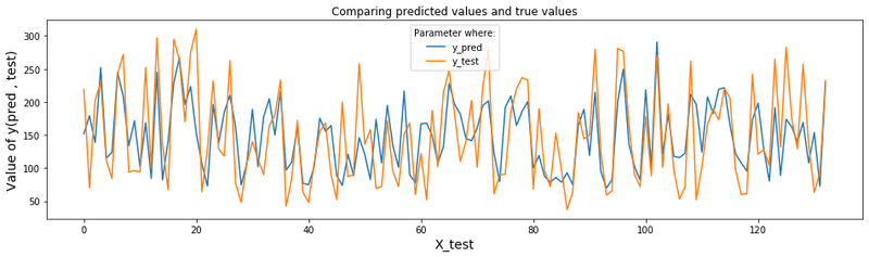
The two lines track each other closely across most of the test range, which is a good qualitative sign before computing a numeric metric.
Evaluating Regression Error
Root Mean Squared Error (RMSE) is the square root of the average squared difference between predicted and true values — it is in the same units as the target. Calculate the RMSE using mean_squared_error():
np.sqrt(metrics.mean_squared_error(y_test, y_pred))53.505825893179875To put this in context, calculate what fraction of the target's standard deviation the error represents:
(72.78-53.50)/72.780.26490794174223686y_test.std()73.47317715932746The RMSE of 53.5 is about 27 % of the target's standard deviation of 73.5, meaning the model explains a meaningful portion of the variance in disease progression — a reasonable baseline result without any hyperparameter tuning.
Random Forest as a Classifier
This section trains a RandomForestClassifier on the Iris dataset — 150 flower samples with four measurements each, split across three species.
Import the classifier and load the dataset:
from sklearn.ensemble import RandomForestClassifieriris = datasets.load_iris()
iris.target_namesarray(['setosa', 'versicolor', 'virginica'], dtype='<U10')Print the dataset description to understand the features and class distribution:
print(iris.DESCR).. _iris_dataset:
Iris plants dataset
--------------------
**Data Set Characteristics:**
:Number of Instances: 150 (50 in each of three classes)
:Number of Attributes: 4 numeric, predictive attributes and the class
:Attribute Information:
- sepal length in cm
- sepal width in cm
- petal length in cm
- petal width in cm
- class:
- Iris-Setosa
- Iris-Versicolour
- Iris-Virginica
:Summary Statistics:
============== ==== ==== ======= ===== ====================
Min Max Mean SD Class Correlation
============== ==== ==== ======= ===== ====================
sepal length: 4.3 7.9 5.84 0.83 0.7826
sepal width: 2.0 4.4 3.05 0.43 -0.4194
petal length: 1.0 6.9 3.76 1.76 0.9490 (high!)
petal width: 0.1 2.5 1.20 0.76 0.9565 (high!)
============== ==== ==== ======= ===== ====================
:Missing Attribute Values: None
:Class Distribution: 33.3% for each of 3 classes.
:Creator: R.A. Fisher
:Donor: Michael Marshall (MARSHALL%PLU@io.arc.nasa.gov)
:Date: July, 1988
The famous Iris database, first used by Sir R.A. Fisher. The dataset is taken
from Fisher's paper. Note that it's the same as in R, but not as in the UCI
Machine Learning Repository, which has two wrong data points.
This is perhaps the best known database to be found in the
pattern recognition literature. Fisher's paper is a classic in the field and
is referenced frequently to this day. (See Duda & Hart, for example.) The
data set contains 3 classes of 50 instances each, where each class refers to a
type of iris plant. One class is linearly separable from the other 2; the
latter are NOT linearly separable from each other.Assign features and target, then split with stratification to preserve the class balance in both sets:
X = iris.data
y = iris.targetX_train, X_test, y_train, y_test = train_test_split(X, y, random_state = 1, test_size = 0.3, stratify = y)Fit the classifier with 100 trees:
clf = RandomForestClassifier(n_estimators=100, random_state = 42)
clf.fit(X_train, y_train)          RandomForestClassifier(random_state=42)
Predicting and Measuring Accuracy
The predict() method assigns the majority-vote class label from all 100 trees to each test sample. Run predictions and print the accuracy score:
y_pred = clf.predict(X_test)
print(metrics.accuracy_score(y_test, y_pred))0.9777777777777777The model achieves 97.8 % accuracy on the 45-sample test set, meaning it misclassified only one flower.
Interpreting the Confusion Matrix
A confusion matrix is a square grid where each cell counts the number of samples from true class that were predicted as class . The diagonal holds correct predictions; off-diagonal cells are mistakes. Compute the raw matrix first:
mat = metrics.confusion_matrix(y_test, y_pred)
matarray([[15, 0, 0],
[ 0, 15, 0],
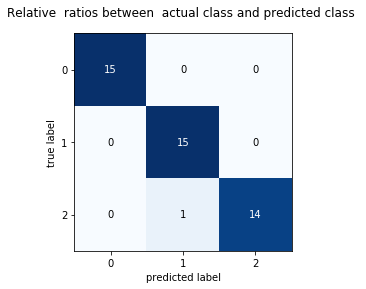
[ 0, 1, 14]], dtype=int64)The classifier was perfect on setosa and versicolor, and misclassified one virginica sample as versicolor. Now plot the matrix as a colour-coded heatmap for easier reading:
from mlxtend.evaluate import confusion_matrix
from mlxtend.plotting import plot_confusion_matrix
print('Confusion Matrix')
cm = confusion_matrix(y_test, y_pred)
fig, ax = plot_confusion_matrix(conf_mat = cm  )
plt.title('Relative  ratios between  actual class and predicted class ')
plt.show()Confusion MatrixThe heatmap below makes it immediately clear that the three diagonal blocks are dark (many correct predictions) and only one off-diagonal cell is non-zero:
Extracting Feature Importances
After training, clf.feature_importances_ returns the mean decrease in Gini impurity for each feature, normalized so that all values sum to 1. Retrieve the array and match it to the feature names:
clf.feature_importances_array([0.1160593 , 0.03098375, 0.43034957, 0.42260737])iris.feature_names['sepal length (cm)', 'sepal width (cm)', 'petal length (cm)', 'petal width (cm)']Petal length (43 %) and petal width (42 %) together account for 85 % of the model's discriminating power. Sepal length contributes a modest 12 %, while sepal width is almost irrelevant at 3 %. This matches the dataset's own correlation statistics, where petal measurements have correlations above 0.95.
Conclusion
In this tutorial you trained a RandomForestRegressor on the 442-sample Diabetes dataset, achieving an RMSE of 53.5 against a target standard deviation of 73.5. You then trained a RandomForestClassifier on the Iris dataset and reached 97.8 % accuracy, misclassifying just one of 45 test samples. Finally, you extracted feature importances and confirmed that petal length and petal width drive almost all of the classifier's decisions.
Key takeaways:
- Random Forest reduces overfitting by training each tree on a different bootstrap sample and restricting each split to a random feature subset — neither trick alone is enough, but together they work well.
- RMSE normalized against the target's standard deviation gives you a quick sense of how much variance the regressor explains without needing R² directly.
- Feature importances are computed from Gini impurity reductions across all trees — they are a fast way to rank features, but can overrate high-cardinality numerical features on some datasets.
- The confusion matrix is your first diagnostic after a classification run: one glance tells you which classes the model confuses and whether errors are symmetric.
Next steps:
- Read Ensemble Learning in Python for a broader look at bagging, boosting, and stacking and how they compare to Random Forest.
- Explore Decision Tree in Python to understand the building block that every tree in the forest is based on.
- Tune your forest by experimenting with
max_features(the fraction of features considered at each split) — reducing it below the default'sqrt'often reduces correlation between trees and improves ensemble accuracy.

