Ensemble Learning in Python

Ensemble learning is the practice of combining multiple machine learning models to produce a prediction that is more accurate and robust than any single model could achieve alone. Instead of relying on one algorithm, you train several and merge their outputs using a statistical rule such as majority voting or averaging.

In this tutorial you will train four ensemble classifiers on the UCI Breast Cancer Wisconsin dataset: RandomForestClassifier, AdaBoostClassifier, GradientBoostingClassifier, and XGBClassifier. You will also explore the theory behind bagging and boosting so you understand which technique to reach for in different situations.

Prerequisites: Python 3.x, scikit-learn, XGBoost, Pandas, NumPy, Matplotlib.

What is Ensemble Learning?

Ensemble learning trains multiple models on the same dataset, collects their individual predictions, and then combines those predictions with a statistical rule to produce a final output. The core idea is that different algorithms have different strengths: where one model fails, another may succeed, so their combined output is more reliable than any one of them individually.

The diagram below shows the general structure of an ensemble: a shared dataset feeds several base learners (Lasso, KNN, SVR, Random Forest), whose outputs flow into a single meta-layer that produces the final prediction.

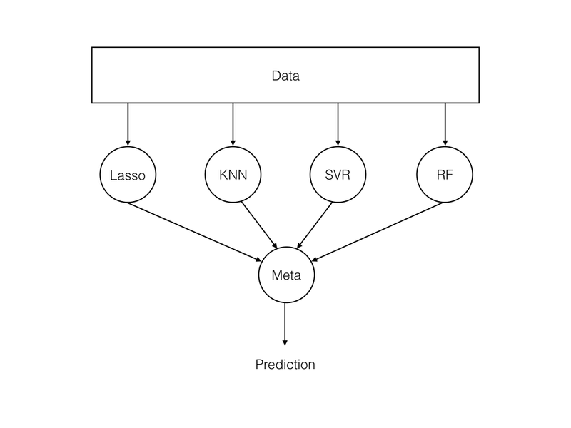
Think of it like a sports team: each player is a specialist, and the team's collective performance exceeds what any individual could accomplish alone. In the same way, each algorithm excels in a particular region of the feature space, and combining them covers each other's blind spots.

Why Ensemble Learning Works

When you start with a single model and push it toward high accuracy, you often end up with either overfitting (low bias, high variance) or underfitting (high bias, low variance). Ensemble methods manage this tradeoff by combining models in ways that specifically target one of these failure modes.

Every machine learning model's error can be decomposed into three components:

• Bias — how far, on average, are your predictions from the true values?
• Variance — how much do predictions change across different training sets?
• Irreducible error — noise in the data that no model can eliminate.

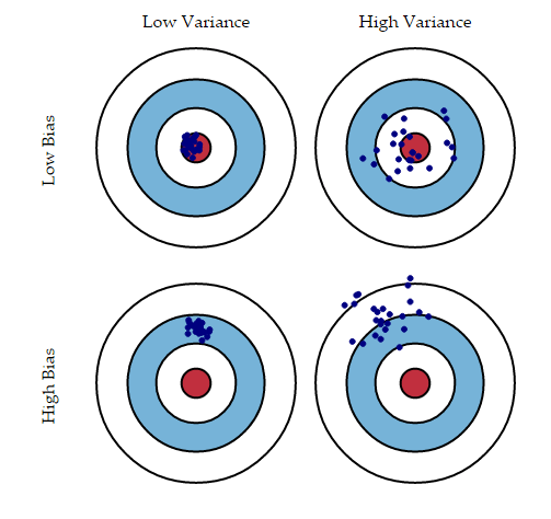
The bull's-eye diagram below illustrates what bias and variance mean in practice: low bias means predictions cluster around the true target; low variance means predictions are consistent with each other across trials.

The bias-variance tradeoff chart below shows how total error behaves as model complexity increases. Simple models (left side) have high bias and low variance; complex models (right side) have low bias and high variance. The optimal model sits at the minimum of the total error curve.

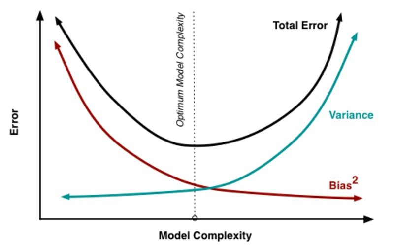
If your model shows high bias, you have room to increase complexity. If it shows high variance, you need to reduce complexity or add regularization. Ensemble methods give you a principled way to navigate this tradeoff.

Types of Ensemble Learning

Ensemble techniques fall into three broad categories depending on how predictions are combined.

Basic Combination Techniques

Max voting is used for classification: each model votes for a class, and the majority class wins. Averaging computes the mean of all model predictions and works well for regression. Weighted averaging extends plain averaging by assigning higher weight to models that have proven more accurate on validation data.

Advanced Ensemble Techniques

More powerful techniques include stacking (training a meta-model on the outputs of base models), blending (a simplified version of stacking with a holdout set), bagging, and boosting. Bagging and boosting are the two most widely used advanced techniques and are covered in detail below.

Bagging

Bagging — short for Bootstrap Aggregating — creates multiple random subsets of the training data by sampling with replacement, trains one model on each subset, and combines their predictions by voting (classification) or averaging (regression). Its primary goal is to reduce variance without increasing bias.

The diagram below shows the bagging workflow: the original dataset is split into five subsets (D1–D5), each trains a separate model, and all model outputs are merged into a single combined prediction.

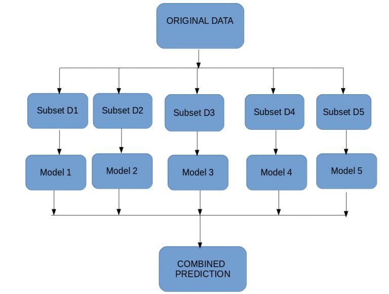
Random Forest is the canonical bagging algorithm. It builds many decision trees on bootstrap samples and at each node selects only a random subset of features to split on, which decorrelates the trees and reduces variance further.

Boosting

Boosting is a sequential process in which each new model is trained to correct the errors left by the previous one. Models are weighted by their performance, so better models contribute more to the final prediction. Its primary goal is to reduce bias rather than variance.

The diagram below illustrates sequential boosting: starting from the original dataset $D_1$, each round updates sample weights so that misclassified points receive more emphasis ($D_2$, $D_3$), and all trained classifiers are combined into a single stronger classifier.

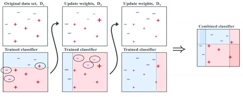
Key properties of boosting compared to bagging:

• Combining predictions that belong to different types of errors (across sequential rounds).
• Aims to decrease bias, not variance.
• Models are weighted according to their individual performance.

Algorithms Available in scikit-learn

scikit-learn and XGBoost provide four ready-to-use ensemble classifiers that cover both the bagging and boosting paradigms:

• Random Forest follows the bagging approach: it fits many decision trees on random bootstrap samples and averages their predictions.
• AdaBoost (Adaptive Boosting) is one of the simplest boosting algorithms: it fits a sequence of weak classifiers, each time upweighting samples that the previous classifier got wrong.
• Gradient Boosting builds an additive model in a forward stage-wise fashion, optimizing a differentiable loss function at each step.
• XGBoost (Extreme Gradient Boosting) is an advanced, highly optimized implementation of gradient boosting that uses a custom DMatrix internal data structure for memory efficiency and training speed.

Data Preparation

Start by importing all required libraries in a single block:

import pandas as pd
import seaborn as sns
import matplotlib.pyplot as plt
import numpy as np
from sklearn import datasets, metrics
from sklearn.model_selection import train_test_split
from sklearn.preprocessing import StandardScaler
from sklearn.ensemble import RandomForestClassifier, AdaBoostClassifier, GradientBoostingClassifier
import xgboost as xgb

Load the breast cancer dataset from scikit-learn's built-in datasets:

cancer = datasets.load_breast_cancer()

Print the full dataset description to understand its structure and feature definitions:

print(cancer.DESCR)

.. _breast_cancer_dataset:

Breast cancer wisconsin (diagnostic) dataset
--------------------------------------------

**Data Set Characteristics:**

    :Number of Instances: 569

    :Number of Attributes: 30 numeric, predictive attributes and the class

    :Attribute Information:
        - radius (mean of distances from center to points on the perimeter)
        - texture (standard deviation of gray-scale values)
        - perimeter
        - area
        - smoothness (local variation in radius lengths)
        - compactness (perimeter^2 / area - 1.0)
        - concavity (severity of concave portions of the contour)
        - concave points (number of concave portions of the contour)
        - symmetry
        - fractal dimension ("coastline approximation" - 1)

        The mean, standard error, and "worst" or largest (mean of the three
        worst/largest values) of these features were computed for each image,
        resulting in 30 features.  For instance, field 0 is Mean Radius, field
        10 is Radius SE, field 20 is Worst Radius.

        - class:
                - WDBC-Malignant
                - WDBC-Benign

    :Summary Statistics:

    ===================================== ====== ======
                                           Min    Max
    ===================================== ====== ======
    radius (mean):                        6.981  28.11
    texture (mean):                       9.71   39.28
    perimeter (mean):                     43.79  188.5
    area (mean):                          143.5  2501.0
    smoothness (mean):                    0.053  0.163
    compactness (mean):                   0.019  0.345
    concavity (mean):                     0.0    0.427
    concave points (mean):                0.0    0.201
    symmetry (mean):                      0.106  0.304
    fractal dimension (mean):             0.05   0.097
    radius (standard error):              0.112  2.873
    texture (standard error):             0.36   4.885
    perimeter (standard error):           0.757  21.98
    area (standard error):                6.802  542.2
    smoothness (standard error):          0.002  0.031
    compactness (standard error):         0.002  0.135
    concavity (standard error):           0.0    0.396
    concave points (standard error):      0.0    0.053
    symmetry (standard error):            0.008  0.079
    fractal dimension (standard error):   0.001  0.03
    radius (worst):                       7.93   36.04
    texture (worst):                      12.02  49.54
    perimeter (worst):                    50.41  251.2
    area (worst):                         185.2  4254.0
    smoothness (worst):                   0.071  0.223
    compactness (worst):                  0.027  1.058
    concavity (worst):                    0.0    1.252
    concave points (worst):               0.0    0.291
    symmetry (worst):                     0.156  0.664
    fractal dimension (worst):            0.055  0.208
    ===================================== ====== ======

    :Missing Attribute Values: None

    :Class Distribution: 212 - Malignant, 357 - Benign

    :Creator:  Dr. William H. Wolberg, W. Nick Street, Olvi L. Mangasarian

    :Donor: Nick Street

    :Date: November, 1995

This is a copy of UCI ML Breast Cancer Wisconsin (Diagnostic) datasets.
https://goo.gl/U2Uwz2

Features are computed from a digitized image of a fine needle
aspirate (FNA) of a breast mass.  They describe
characteristics of the cell nuclei present in the image.

Separating plane described above was obtained using
Multisurface Method-Tree (MSM-T) [K. P. Bennett, "Decision Tree
Construction Via Linear Programming." Proceedings of the 4th
Midwest Artificial Intelligence and Cognitive Science Society,
pp. 97-101, 1992], a classification method which uses linear
programming to construct a decision tree.  Relevant features
were selected using an exhaustive search in the space of 1-4
features and 1-3 separating planes.

The actual linear program used to obtain the separating plane
in the 3-dimensional space is that described in:
[K. P. Bennett and O. L. Mangasarian: "Robust Linear
Programming Discrimination of Two Linearly Inseparable Sets",
Optimization Methods and Software 1, 1992, 23-34].

Extract the feature matrix X and target vector y from the dataset object:

X = cancer.data
y = cancer.target

Confirm the dataset contains 569 samples and 30 features:

X.shape, y.shape

((569, 30), (569,))

The 30 features span very different scales — some in the tens, others in the hundreds. Standardize the data using StandardScaler so that no single feature dominates due to its magnitude:

scaler = StandardScaler()
X_scaled = scaler.fit_transform(X)
X_scaled[: 2]

array([[ 1.09706398e+00, -2.07333501e+00,  1.26993369e+00,
         9.84374905e-01,  1.56846633e+00,  3.28351467e+00,
         2.65287398e+00,  2.53247522e+00,  2.21751501e+00,
         2.25574689e+00,  2.48973393e+00, -5.65265059e-01,
         2.83303087e+00,  2.48757756e+00, -2.14001647e-01,
         1.31686157e+00,  7.24026158e-01,  6.60819941e-01,
         1.14875667e+00,  9.07083081e-01,  1.88668963e+00,
        -1.35929347e+00,  2.30360062e+00,  2.00123749e+00,
         1.30768627e+00,  2.61666502e+00,  2.10952635e+00,
         2.29607613e+00,  2.75062224e+00,  1.93701461e+00],
       [ 1.82982061e+00, -3.53632408e-01,  1.68595471e+00,
         1.90870825e+00, -8.26962447e-01, -4.87071673e-01,
        -2.38458552e-02,  5.48144156e-01,  1.39236330e-03,
        -8.68652457e-01,  4.99254601e-01, -8.76243603e-01,
         2.63326966e-01,  7.42401948e-01, -6.05350847e-01,
        -6.92926270e-01, -4.40780058e-01,  2.60162067e-01,
        -8.05450380e-01, -9.94437403e-02,  1.80592744e+00,
        -3.69203222e-01,  1.53512599e+00,  1.89048899e+00,
        -3.75611957e-01, -4.30444219e-01, -1.46748968e-01,
         1.08708430e+00, -2.43889668e-01,  2.81189987e-01]])

After scaling, each feature has zero mean and unit variance, which prevents algorithms sensitive to feature magnitude (such as KNN or SVMs) from being dominated by large-scale attributes.

Training the Ensemble Classifiers

Instantiate all four classifiers with 200 estimators and a fixed random seed so results are reproducible. Gradient Boosting and AdaBoost also use a low learning_rate of 0.01 to keep each step conservative and reduce overfitting:

rfc = RandomForestClassifier(n_estimators=200, random_state=1)
abc = AdaBoostClassifier(n_estimators=200, random_state= 1, learning_rate=0.01)
gbc = GradientBoostingClassifier(n_estimators=200, random_state=1, learning_rate=0.01)
xgb_clf = xgb.XGBClassifier(n_estimators=200, learning_rate=0.01, random_state=1)

Split the scaled data into 80 % training and 20 % test sets, using stratify=y to preserve the class distribution in both splits:

X_train, X_test, y_train, y_test = train_test_split(X_scaled, y, test_size = 0.2, random_state = 1, stratify = y)

Fit all four classifiers on the training data:

rfc.fit(X_train, y_train)
abc.fit(X_train, y_train)
gbc.fit(X_train, y_train)
xgb_clf.fit(X_train, y_train)

The XGBoost classifier prints its full configuration when training completes, confirming the hyperparameters used:

XGBClassifier(base_score=0.5, booster='gbtree', colsample_bylevel=1,
              colsample_bynode=1, colsample_bytree=1, gamma=0, gpu_id=-1,
              importance_type='gain', interaction_constraints='',
              learning_rate=0.01, max_delta_step=0, max_depth=6,
              min_child_weight=1, missing=nan, monotone_constraints='()',
              n_estimators=200, n_jobs=0, num_parallel_tree=1, random_state=1,
              reg_alpha=0, reg_lambda=1, scale_pos_weight=1, subsample=1,
              tree_method='exact', validate_parameters=1, verbosity=None)

Comparing Model Accuracy

Evaluate each classifier on the held-out test set and print accuracy scores side by side:

print('Random Forest: ', rfc.score(X_test, y_test))
print('AdaBoost: ', abc.score(X_test, y_test))
print('Gradient Boost: ', gbc.score(X_test, y_test))
print('XGBoost: ', xgb_clf.score(X_test, y_test))

Random Forest:  0.9473684210526315
AdaBoost:  0.9473684210526315
Gradient Boost:  0.9736842105263158
XGBoost:  0.9649122807017544

Gradient Boosting leads the comparison at approximately 97.4 % accuracy, followed by XGBoost at 96.5 % and both Random Forest and AdaBoost at 94.7 %. All four ensemble classifiers outperform the typical single-model baseline on this dataset, and the boosting-based methods edge ahead — consistent with their ability to iteratively correct prediction errors.

Conclusion

In this tutorial you trained four ensemble classifiers — Random Forest, AdaBoost, Gradient Boosting, and XGBoost — on the breast cancer dataset. After standardizing the 30 features and performing an 80/20 stratified split, Gradient Boosting reached the highest accuracy at 97.4 %, while all four models comfortably exceeded 94 % — demonstrating that combining multiple learners consistently beats any single-model approach on this classification task.

Key takeaways:

• Ensemble learning reduces prediction error by combining the strengths of multiple base models rather than relying on one.
• Bagging (Random Forest) targets variance reduction by training independent models on bootstrap samples in parallel.
• Boosting (AdaBoost, Gradient Boosting, XGBoost) targets bias reduction by training models sequentially, each correcting the errors of the previous one.
• Standardizing features before ensemble training is important for algorithms that use distance or gradient information under the hood.
• A low learning_rate with many estimators generally outperforms a high rate with fewer — but increases training time.

Next steps:

• Explore Random Forest Classifier and Regressor for a deeper dive into how the bagging-based forest algorithm works and how to tune its hyperparameters.
• Read Improve Training Time Using Bagging to see how the bagging meta-estimator can wrap any base learner and speed up training through parallelism.
• Experiment with the n_estimators and learning_rate parameters across all four classifiers on your own dataset, and use feature_importances_ to understand which features each ensemble relies on most.