
Picking the right features is often the difference between a model that generalises well and one that overfits on noise. Wrapper methods — a family of feature selection techniques — take a direct approach: they train an actual machine learning model on candidate subsets and use that model's performance as the selection criterion.
Unlike filter methods (which score features independently using statistics), wrapper methods capture the way features interact with each other. The trade-off is computation time: every candidate subset requires a full model training run. For this reason, wrapper methods are best suited to datasets with a moderate number of features (tens rather than hundreds).
In this tutorial you will apply three wrapper strategies — Sequential Forward Selection, Sequential Backward Selection, and Exhaustive Feature Selection — to scikit-learn's Wine dataset using the mlxtend library. You will compare which subset each strategy selects and what cross-validation accuracy it achieves.
Prerequisites: Python 3.x, scikit-learn, mlxtend, Pandas, NumPy, Matplotlib.
What Are Wrapper Methods?
A wrapper method works by treating the feature subset as a search problem. It repeatedly generates a candidate subset, feeds it into a learning algorithm, measures performance, and uses that performance signal to decide which subset to try next.
The diagram below shows the core loop: all features enter on the left, a candidate subset is generated, a learning algorithm evaluates it, and the resulting performance score drives the next iteration.
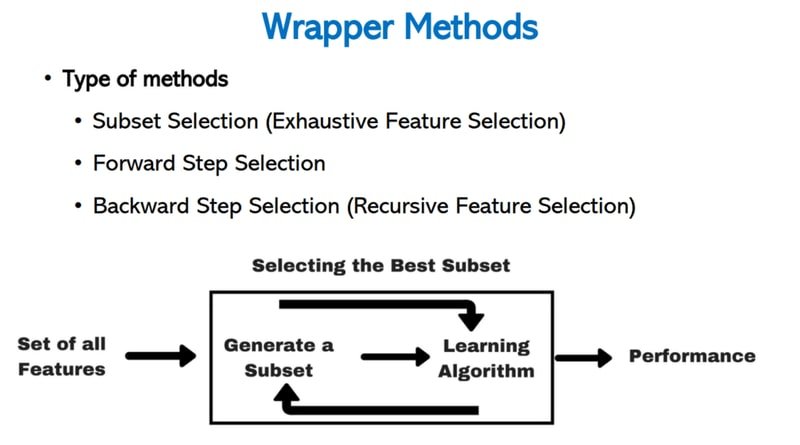
Three search strategies fall under this umbrella:
- Subset Selection (Exhaustive Feature Selection) — evaluate every possible subset
- Forward Step Selection — start empty, add one feature at a time
- Backward Step Selection — start with all features, remove one at a time
Sequential Forward Selection (SFS)
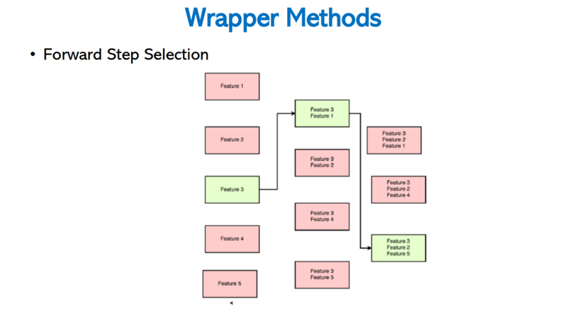
Sequential Forward Selection begins with an empty set and greedily adds the one feature that gives the biggest performance gain at each step. It keeps adding features until the target subset size is reached.
The diagram below illustrates how, starting from individual features, the algorithm selects the best single feature (Feature 3, shown in green) and then expands the winning subset step by step:
Sequential Backward Selection (SBS)
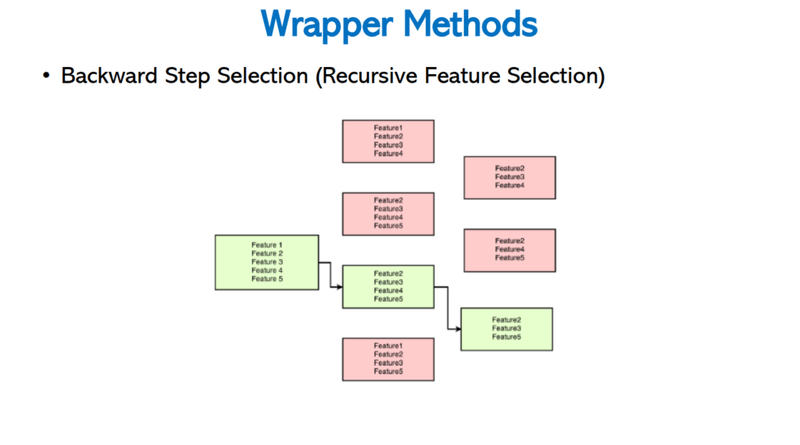
Sequential Backward Selection is the mirror image of SFS. It begins with the full feature set and greedily removes the feature whose absence costs the least performance. This continues until only features remain.
The diagram below shows the pruning process: starting from all five features (green box, left), the algorithm removes one feature per step until it reaches the best small subset (rightmost green box):
Exhaustive Feature Selection (EFS)
Exhaustive Feature Selection (also called best-subset selection) evaluates every possible combination of features. It is guaranteed to find the globally optimal subset, but the number of subsets grows exponentially: for features there are combinations. For this reason, EFS is only practical when the feature count is small or when a bounded range of subset sizes is specified.
How mlxtend Implements These Algorithms
mlxtend is an open-source Python library that provides SequentialFeatureSelector and ExhaustiveFeatureSelector. Both classes accept any scikit-learn-compatible estimator and support parallel execution via n_jobs.
Install mlxtend if you have not already:
!pip install mlxtendThe command above produces output like the following, confirming the install and its dependencies:
Requirement already satisfied: mlxtend in c:\users\srish\appdata\roaming\python\python38\site-packages (0.17.3)
Requirement already satisfied: scikit-learn>=0.20.3 in e:\callme_conda\lib\site-packages (from mlxtend) (0.23.1)
Requirement already satisfied: pandas>=0.24.2 in e:\callme_conda\lib\site-packages (from mlxtend) (1.0.5)
Requirement already satisfied: joblib>=0.13.2 in e:\callme_conda\lib\site-packages (from mlxtend) (0.16.0)
Requirement already satisfied: matplotlib>=3.0.0 in e:\callme_conda\lib\site-packages (from mlxtend) (3.2.2)
Requirement already satisfied: setuptools in e:\callme_conda\lib\site-packages (from mlxtend) (49.2.0.post20200714)
Requirement already satisfied: numpy>=1.16.2 in e:\callme_conda\lib\site-packages (from mlxtend) (1.18.5)
Requirement already satisfied: scipy>=1.2.1 in e:\callme_conda\lib\site-packages (from mlxtend) (1.5.0)
Requirement already satisfied: threadpoolctl>=2.0.0 in e:\callme_conda\lib\site-packages (from scikit-learn>=0.20.3->mlxtend) (2.1.0)
Requirement already satisfied: python-dateutil>=2.6.1 in e:\callme_conda\lib\site-packages (from pandas>=0.24.2->mlxtend) (2.8.1)
Requirement already satisfied: pytz>=2017.2 in e:\callme_conda\lib\site-packages (from pandas>=0.24.2->mlxtend) (2020.1)
Requirement already satisfied: cycler>=0.10 in e:\callme_conda\lib\site-packages (from matplotlib>=3.0.0->mlxtend) (0.10.0)
Requirement already satisfied: kiwisolver>=1.0.1 in e:\callme_conda\lib\site-packages (from matplotlib>=3.0.0->mlxtend) (1.2.0)
Requirement already satisfied: pyparsing!=2.0.4,!=2.1.2,!=2.1.6,>=2.0.1 in e:\callme_conda\lib\site-packages (from matplotlib>=3.0.0->mlxtend) (2.4.7)
Requirement already satisfied: six>=1.5 in e:\callme_conda\lib\site-packages (from python-dateutil>=2.6.1->pandas>=0.24.2->mlxtend) (1.15.0)
For full API documentation visit the mlxtend official documentation.
The SequentialFeatureSelector (abbreviated SFS / SBS depending on direction) supports four variants:
- Sequential Forward Selection (SFS) —
forward=True, floating=False - Sequential Backward Selection (SBS) —
forward=False, floating=False - Sequential Forward Floating Selection (SFFS) —
forward=True, floating=True - Sequential Backward Floating Selection (SBFS) —
forward=False, floating=True
All four reduce an initial -dimensional feature space to a -dimensional subspace where , adding or removing one feature per iteration based on classifier performance.
Loading and Preparing the Wine Dataset
Import all the libraries you will need for this tutorial in a single block:
import numpy as np
import pandas as pd
import seaborn as sns
import matplotlib.pyplot as plt
%matplotlib inlinefrom sklearn.model_selection import train_test_split
from sklearn.ensemble import RandomForestRegressor, RandomForestClassifier
from sklearn.metrics import roc_auc_score
from mlxtend.feature_selection import SequentialFeatureSelector as SFSfrom sklearn.datasets import load_wine
from sklearn.preprocessing import StandardScalerLoad the Wine dataset — a classic multi-class classification benchmark where 178 wine samples are described by 13 chemical measurements and labelled into one of three cultivar classes:
data = load_wine()Inspect the dataset's top-level keys:
data.keys()dict_keys(['data', 'target', 'frame', 'target_names', 'DESCR', 'feature_names'])Print the full dataset description to see the feature list and summary statistics:
print(data.DESCR).. _wine_dataset:
Wine recognition dataset
------------------------
**Data Set Characteristics:**
:Number of Instances: 178 (50 in each of three classes)
:Number of Attributes: 13 numeric, predictive attributes and the class
:Attribute Information:
- Alcohol
- Malic acid
- Ash
- Alcalinity of ash
- Magnesium
- Total phenols
- Flavanoids
- Nonflavanoid phenols
- Proanthocyanins
- Color intensity
- Hue
- OD280/OD315 of diluted wines
- Proline
- class:
- class_0
- class_1
- class_2
:Summary Statistics:
============================= ==== ===== ======= =====
Min Max Mean SD
============================= ==== ===== ======= =====
Alcohol: 11.0 14.8 13.0 0.8
Malic Acid: 0.74 5.80 2.34 1.12
Ash: 1.36 3.23 2.36 0.27
Alcalinity of Ash: 10.6 30.0 19.5 3.3
Magnesium: 70.0 162.0 99.7 14.3
Total Phenols: 0.98 3.88 2.29 0.63
Flavanoids: 0.34 5.08 2.03 1.00
Nonflavanoid Phenols: 0.13 0.66 0.36 0.12
Proanthocyanins: 0.41 3.58 1.59 0.57
Colour Intensity: 1.3 13.0 5.1 2.3
Hue: 0.48 1.71 0.96 0.23
OD280/OD315 of diluted wines: 1.27 4.00 2.61 0.71
Proline: 278 1680 746 315
============================= ==== ===== ======= =====
:Missing Attribute Values: None
:Class Distribution: class_0 (59), class_1 (71), class_2 (48)
:Creator: R.A. Fisher
:Donor: Michael Marshall (MARSHALL%PLU@io.arc.nasa.gov)
:Date: July, 1988
This is a copy of UCI ML Wine recognition datasets.
https://archive.ics.uci.edu/ml/machine-learning-databases/wine/wine.data
The data is the results of a chemical analysis of wines grown in the same region in Italy by three different cultivators. There are thirteen differentmeasurements taken for different constituents found in the three types of wine.Place the feature matrix in a DataFrame and the target vector in y:
X = pd.DataFrame(data.data)
y = data.target
Assign column names and preview the first five rows:
X.columns = data.feature_names
X.head()| alcohol | malic_acid | ash | alcalinity_of_ash | magnesium | total_phenols | flavanoids | nonflavanoid_phenols | proanthocyanins | color_intensity | hue | od280/od315_of_diluted_wines | proline | |
|---|---|---|---|---|---|---|---|---|---|---|---|---|---|
| 0 | 14.23 | 1.71 | 2.43 | 15.6 | 127.0 | 2.80 | 3.06 | 0.28 | 2.29 | 5.64 | 1.04 | 3.92 | 1065.0 |
| 1 | 13.20 | 1.78 | 2.14 | 11.2 | 100.0 | 2.65 | 2.76 | 0.26 | 1.28 | 4.38 | 1.05 | 3.40 | 1050.0 |
| 2 | 13.16 | 2.36 | 2.67 | 18.6 | 101.0 | 2.80 | 3.24 | 0.30 | 2.81 | 5.68 | 1.03 | 3.17 | 1185.0 |
| 3 | 14.37 | 1.95 | 2.50 | 16.8 | 113.0 | 3.85 | 3.49 | 0.24 | 2.18 | 7.80 | 0.86 | 3.45 | 1480.0 |
| 4 | 13.24 | 2.59 | 2.87 | 21.0 | 118.0 | 2.80 | 2.69 | 0.39 | 1.82 | 4.32 | 1.04 | 2.93 | 735.0 |
Check for missing values — the Wine dataset is clean, but it is good practice to confirm:
X.isnull().sum()alcohol 0
malic_acid 0
ash 0
alcalinity_of_ash 0
magnesium 0
total_phenols 0
flavanoids 0
nonflavanoid_phenols 0
proanthocyanins 0
color_intensity 0
hue 0
od280/od315_of_diluted_wines 0
proline 0
dtype: int64All 13 features have zero missing values. Split into 80 % training and 20 % test sets:
X_train, X_test, y_train, y_test = train_test_split(X, y, test_size = 0.2, random_state = 0)
X_train.shape, X_test.shape((142, 13), (36, 13))The training set has 142 samples and the test set has 36 samples, each with 13 features.
Step Forward Feature Selection (SFS)
Selecting a Fixed Number of Features
SequentialFeatureSelector wraps any scikit-learn estimator. Pass forward=True to enable forward selection. The k_features parameter sets the exact number of features to select, cv=4 applies 4-fold cross-validation on the training set, and n_jobs=-1 uses all available CPU cores:
sfs = SFS(RandomForestClassifier(n_estimators=100, random_state=0, n_jobs = -1),
         k_features = 7,
          forward= True,
          floating = False,
          verbose= 2,
          scoring= 'accuracy',
          cv = 4,
          n_jobs= -1
         ).fit(X_train, y_train)
The verbose log below shows the cross-validated accuracy at each step as features are added one by one, from 1 feature up to the target of 7:
[Parallel(n_jobs=-1)]: Using backend LokyBackend with 8 concurrent workers.
[Parallel(n_jobs=-1)]: Done   5 out of  13 | elapsed:    4.2s remaining:    6.8s
[Parallel(n_jobs=-1)]: Done  13 out of  13 | elapsed:    5.8s finished

[2020-08-06 12:56:29] Features: 1/7 -- score: 0.7674603174603174[Parallel(n_jobs=-1)]: Using backend LokyBackend with 8 concurrent workers.
[Parallel(n_jobs=-1)]: Done   4 out of  12 | elapsed:    1.5s remaining:    3.1s
[Parallel(n_jobs=-1)]: Done  12 out of  12 | elapsed:    3.2s finished

[2020-08-06 12:56:33] Features: 2/7 -- score: 0.9718253968253968[Parallel(n_jobs=-1)]: Using backend LokyBackend with 8 concurrent workers.
[Parallel(n_jobs=-1)]: Done   2 out of  11 | elapsed:    2.3s remaining:   10.6s
[Parallel(n_jobs=-1)]: Done   8 out of  11 | elapsed:    2.8s remaining:    1.0s
[Parallel(n_jobs=-1)]: Done  11 out of  11 | elapsed:    4.7s finished

[2020-08-06 12:56:37] Features: 3/7 -- score: 0.9859126984126985[Parallel(n_jobs=-1)]: Using backend LokyBackend with 8 concurrent workers.
[Parallel(n_jobs=-1)]: Done   7 out of  10 | elapsed:    2.2s remaining:    0.9s
[Parallel(n_jobs=-1)]: Done  10 out of  10 | elapsed:    4.5s finished

[2020-08-06 12:56:42] Features: 4/7 -- score: 0.9789682539682539[Parallel(n_jobs=-1)]: Using backend LokyBackend with 8 concurrent workers.
[Parallel(n_jobs=-1)]: Done   4 out of   9 | elapsed:    2.3s remaining:    2.8s
[Parallel(n_jobs=-1)]: Done   9 out of   9 | elapsed:    4.1s remaining:    0.0s
[Parallel(n_jobs=-1)]: Done   9 out of   9 | elapsed:    4.1s finished

[2020-08-06 12:56:46] Features: 5/7 -- score: 0.9720238095238095[Parallel(n_jobs=-1)]: Using backend LokyBackend with 8 concurrent workers.
[Parallel(n_jobs=-1)]: Done   3 out of   8 | elapsed:    2.1s remaining:    3.6s
[Parallel(n_jobs=-1)]: Done   8 out of   8 | elapsed:    2.9s remaining:    0.0s
[Parallel(n_jobs=-1)]: Done   8 out of   8 | elapsed:    2.9s finished

[2020-08-06 12:56:49] Features: 6/7 -- score: 0.9789682539682539[Parallel(n_jobs=-1)]: Using backend LokyBackend with 8 concurrent workers.
[Parallel(n_jobs=-1)]: Done   4 out of   7 | elapsed:    2.3s remaining:    1.7s
[Parallel(n_jobs=-1)]: Done   7 out of   7 | elapsed:    2.7s finished

[2020-08-06 12:56:52] Features: 7/7 -- score: 0.9791666666666666
Retrieve the names of the 7 selected features:
sfs.k_feature_names_('alcohol', 'ash', 'magnesium', 'flavanoids', 'proanthocyanins', 'color_intensity', 'proline')Retrieve their column indices in the original DataFrame:
sfs.k_feature_idx_(0, 2, 4, 6, 8, 9, 12)Check the cross-validated accuracy of the final 7-feature subset:
sfs.k_score_0.9791666666666666A score of approximately 97.9 % with just 7 of the original 13 features is a strong result. You can view the full per-step metrics table:
pd.DataFrame.from_dict(sfs.get_metric_dict()).T| feature_idx | cv_scores | avg_score | feature_names | ci_bound | std_dev | std_err | |
|---|---|---|---|---|---|---|---|
| 1 | (6,) | [0.7222222222222222, 0.8333333333333334, 0.742... | 0.76746 | (flavanoids,) | 0.0670901 | 0.0418533 | 0.024164 |
| 2 | (6, 9) | [0.9444444444444444, 1.0, 0.9714285714285714, ... | 0.971825 | (flavanoids, color_intensity) | 0.031492 | 0.0196459 | 0.0113425 |
| 3 | (4, 6, 9) | [0.9722222222222222, 1.0, 0.9714285714285714, ... | 0.985913 | (magnesium, flavanoids, color_intensity) | 0.0225862 | 0.0140901 | 0.00813492 |
| 4 | (4, 6, 9, 12) | [0.9722222222222222, 0.9722222222222222, 0.971... | 0.978968 | (magnesium, flavanoids, color_intensity, proline) | 0.0194714 | 0.012147 | 0.00701308 |
| 5 | (2, 4, 6, 9, 12) | [0.9444444444444444, 0.9722222222222222, 0.971... | 0.972024 | (ash, magnesium, flavanoids, color_intensity, ... | 0.0314903 | 0.0196449 | 0.011342 |
| 6 | (2, 4, 6, 8, 9, 12) | [0.9722222222222222, 0.9722222222222222, 0.971... | 0.978968 | (ash, magnesium, flavanoids, proanthocyanins, ... | 0.0194714 | 0.012147 | 0.00701308 |
| 7 | (0, 2, 4, 6, 8, 9, 12) | [0.9444444444444444, 0.9722222222222222, 1.0, ... | 0.979167 | (alcohol, ash, magnesium, flavanoids, proantho... | 0.0369201 | 0.0230321 | 0.0132976 |
Notice that the 3-feature subset (magnesium, flavanoids, color_intensity) already achieves 98.6 % — adding more features does not consistently improve accuracy because of the Random Forest's inherent feature importance weighting.
Letting SFS Choose the Best Size Automatically
Instead of fixing k_features to a single integer, you can pass a range tuple (min, max) and let the algorithm select the subset size that achieves the highest cross-validated score within that range:
sfs = SFS(RandomForestClassifier(n_estimators=100, random_state=0, n_jobs = -1),
         k_features = (1, 8),
          forward= True,
          floating = False,
          verbose= 2,
          scoring= 'accuracy',
          cv = 4,
          n_jobs= -1
).fit(X_train, y_train)[Parallel(n_jobs=-1)]: Using backend LokyBackend with 8 concurrent workers.
[Parallel(n_jobs=-1)]: Done 5 out of 13 | elapsed: 2.4s remaining: 4.0s
[Parallel(n_jobs=-1)]: Done 13 out of 13 | elapsed: 4.8s finished
[2020-08-06 12:57:09] Features: 1/8 -- score: 0.7674603174603174[Parallel(n_jobs=-1)]: Using backend LokyBackend with 8 concurrent workers.
[Parallel(n_jobs=-1)]: Done 4 out of 12 | elapsed: 2.3s remaining: 4.7s
[Parallel(n_jobs=-1)]: Done 12 out of 12 | elapsed: 4.4s finished
[2020-08-06 12:57:13] Features: 2/8 -- score: 0.9718253968253968[Parallel(n_jobs=-1)]: Using backend LokyBackend with 8 concurrent workers.
[Parallel(n_jobs=-1)]: Done 2 out of 11 | elapsed: 1.9s remaining: 8.7s
[Parallel(n_jobs=-1)]: Done 8 out of 11 | elapsed: 2.3s remaining: 0.8s
[Parallel(n_jobs=-1)]: Done 11 out of 11 | elapsed: 4.3s finished
[2020-08-06 12:57:17] Features: 3/8 -- score: 0.9859126984126985[Parallel(n_jobs=-1)]: Using backend LokyBackend with 8 concurrent workers.
[Parallel(n_jobs=-1)]: Done 7 out of 10 | elapsed: 2.6s remaining: 1.0s
[Parallel(n_jobs=-1)]: Done 10 out of 10 | elapsed: 4.4s finished
[2020-08-06 12:57:22] Features: 4/8 -- score: 0.9789682539682539[Parallel(n_jobs=-1)]: Using backend LokyBackend with 8 concurrent workers.
[Parallel(n_jobs=-1)]: Done 4 out of 9 | elapsed: 2.5s remaining: 3.1s
[Parallel(n_jobs=-1)]: Done 9 out of 9 | elapsed: 4.3s remaining: 0.0s
[Parallel(n_jobs=-1)]: Done 9 out of 9 | elapsed: 4.3s finished
[2020-08-06 12:57:26] Features: 5/8 -- score: 0.9720238095238095[Parallel(n_jobs=-1)]: Using backend LokyBackend with 8 concurrent workers.
[Parallel(n_jobs=-1)]: Done 3 out of 8 | elapsed: 2.1s remaining: 3.5s
[Parallel(n_jobs=-1)]: Done 8 out of 8 | elapsed: 2.5s remaining: 0.0s
[Parallel(n_jobs=-1)]: Done 8 out of 8 | elapsed: 2.5s finished
[2020-08-06 12:57:29] Features: 6/8 -- score: 0.9789682539682539[Parallel(n_jobs=-1)]: Using backend LokyBackend with 8 concurrent workers.
[Parallel(n_jobs=-1)]: Done 4 out of 7 | elapsed: 1.7s remaining: 1.3s
[Parallel(n_jobs=-1)]: Done 7 out of 7 | elapsed: 1.8s finished
[2020-08-06 12:57:31] Features: 7/8 -- score: 0.9791666666666666[Parallel(n_jobs=-1)]: Using backend LokyBackend with 8 concurrent workers.
[Parallel(n_jobs=-1)]: Done 3 out of 6 | elapsed: 1.9s remaining: 1.9s
[Parallel(n_jobs=-1)]: Done 6 out of 6 | elapsed: 1.9s finished
[2020-08-06 12:57:33] Features: 8/8 -- score: 0.9791666666666666When the selector is free to pick the best size within the range, it returns the subset with the highest score seen during the search:
sfs.k_score_0.9859126984126985The best score of 98.6 % corresponds to the 3-feature subset that was discovered at step 3 of the forward search. Confirm which features were chosen:
sfs.k_feature_names_('magnesium', 'flavanoids', 'color_intensity')With only 3 features, the Random Forest achieves a higher cross-validated accuracy than with 7 features — a clear demonstration that adding more features does not always help.
Step Backward Selection (SBS)
Step Backward Selection uses the same SequentialFeatureSelector class, but with forward=False. The algorithm starts from all 13 features and eliminates one at a time, keeping the subset that loses the least performance at each step:
sfs = SFS(RandomForestClassifier(n_estimators=100, random_state=0, n_jobs = -1),
         k_features = (1, 8),
          forward= False,
          floating = False,
          verbose= 2,
          scoring= 'accuracy',
          cv = 4,
          n_jobs= -1
         ).fit(X_train, y_train)
The log counts down from 12 features to 1, reporting the cross-validated score at each pruning step:
[Parallel(n_jobs=-1)]: Using backend LokyBackend with 8 concurrent workers.
[Parallel(n_jobs=-1)]: Done   5 out of  13 | elapsed:    2.2s remaining:    3.6s
[Parallel(n_jobs=-1)]: Done  13 out of  13 | elapsed:    4.6s finished

[2020-08-06 12:57:54] Features: 12/1 -- score: 0.9861111111111112[Parallel(n_jobs=-1)]: Using backend LokyBackend with 8 concurrent workers.
[Parallel(n_jobs=-1)]: Done   4 out of  12 | elapsed:    2.2s remaining:    4.5s
[Parallel(n_jobs=-1)]: Done  12 out of  12 | elapsed:    4.5s finished

[2020-08-06 12:57:58] Features: 11/1 -- score: 0.9861111111111112[Parallel(n_jobs=-1)]: Using backend LokyBackend with 8 concurrent workers.
[Parallel(n_jobs=-1)]: Done   2 out of  11 | elapsed:    2.2s remaining:   10.3s
[Parallel(n_jobs=-1)]: Done   8 out of  11 | elapsed:    2.7s remaining:    0.9s
[Parallel(n_jobs=-1)]: Done  11 out of  11 | elapsed:    4.1s finished

[2020-08-06 12:57:58] Features: 10/1 -- score: 0.9791666666666666[Parallel(n_jobs=-1)]: Using backend LokyBackend with 8 concurrent workers.
[Parallel(n_jobs=-1)]: Done   7 out of  10 | elapsed:    3.1s remaining:    1.3s
[Parallel(n_jobs=-1)]: Done  10 out of  10 | elapsed:    4.9s finished

[2020-08-06 12:58:08] Features: 9/1 -- score: 0.9861111111111112[Parallel(n_jobs=-1)]: Using backend LokyBackend with 8 concurrent workers.
[Parallel(n_jobs=-1)]: Done   4 out of   9 | elapsed:    2.1s remaining:    2.7s
[Parallel(n_jobs=-1)]: Done   9 out of   9 | elapsed:    4.1s remaining:    0.0s
[Parallel(n_jobs=-1)]: Done   9 out of   9 | elapsed:    4.1s finished

[2020-08-06 12:58:12] Features: 8/1 -- score: 0.9859126984126985[Parallel(n_jobs=-1)]: Using backend LokyBackend with 8 concurrent workers.
[Parallel(n_jobs=-1)]: Done   3 out of   8 | elapsed:    2.2s remaining:    3.8s
[Parallel(n_jobs=-1)]: Done   8 out of   8 | elapsed:    2.7s remaining:    0.0s
[Parallel(n_jobs=-1)]: Done   8 out of   8 | elapsed:    2.7s finished

[2020-08-06 12:58:15] Features: 7/1 -- score: 0.978968253968254[Parallel(n_jobs=-1)]: Using backend LokyBackend with 8 concurrent workers.
[Parallel(n_jobs=-1)]: Done   4 out of   7 | elapsed:    2.1s remaining:    1.6s
[Parallel(n_jobs=-1)]: Done   7 out of   7 | elapsed:    2.4s finished

[2020-08-06 12:58:17] Features: 6/1 -- score: 0.9859126984126985[Parallel(n_jobs=-1)]: Using backend LokyBackend with 8 concurrent workers.
[Parallel(n_jobs=-1)]: Done   3 out of   6 | elapsed:    1.7s remaining:    1.7s
[Parallel(n_jobs=-1)]: Done   6 out of   6 | elapsed:    1.8s finished

[2020-08-06 12:58:19] Features: 5/1 -- score: 0.9789682539682539[Parallel(n_jobs=-1)]: Using backend LokyBackend with 8 concurrent workers.
[Parallel(n_jobs=-1)]: Done   2 out of   5 | elapsed:    2.1s remaining:    3.2s
[Parallel(n_jobs=-1)]: Done   5 out of   5 | elapsed:    2.1s remaining:    0.0s
[Parallel(n_jobs=-1)]: Done   5 out of   5 | elapsed:    2.1s finished

[2020-08-06 12:58:21] Features: 4/1 -- score: 0.9718253968253968[Parallel(n_jobs=-1)]: Using backend LokyBackend with 8 concurrent workers.
[Parallel(n_jobs=-1)]: Done   4 out of   4 | elapsed:    2.3s remaining:    0.0s
[Parallel(n_jobs=-1)]: Done   4 out of   4 | elapsed:    2.3s finished

[2020-08-06 12:58:24] Features: 3/1 -- score: 0.9718253968253968[Parallel(n_jobs=-1)]: Using backend LokyBackend with 8 concurrent workers.
[Parallel(n_jobs=-1)]: Done   3 out of   3 | elapsed:    2.3s finished

[2020-08-06 12:58:26] Features: 2/1 -- score: 0.9718253968253968[Parallel(n_jobs=-1)]: Using backend LokyBackend with 8 concurrent workers.
[Parallel(n_jobs=-1)]: Done   2 out of   2 | elapsed:    2.2s finished

[2020-08-06 12:58:28] Features: 1/1 -- score: 0.7674603174603174
Assign the result to sbs for clarity and check its best score:
sbs = sfs
sbs.k_score_0.9859126984126985Retrieve the names of the features retained by SBS:
sbs.k_feature_names_('alcohol', 'malic_acid', 'ash', 'alcalinity_of_ash', 'magnesium', 'flavanoids', 'nonflavanoid_phenols', 'color_intensity')SBS selects 8 features with a cross-validated accuracy of 98.6 % — the same peak score as SFS, but with a larger subset. This is typical of greedy backward search: it tends to retain more features than forward search because removing a feature that seems redundant in a large set may still hurt performance when the set is small.
Exhaustive Feature Selection (EFS)
How Many Subsets Are There?
The total number of subsets for features is . For 13 features that is subsets — feasible if a size range is specified. The number of subsets of size exactly from features is the binomial coefficient:
Where:
- — total number of features in the dataset
- — size of the subset being evaluated
- — factorial operator
Bounding the search to subsets of size 4 or 5 gives:
This is a tractable number even on a laptop.
Running EFS
Import ExhaustiveFeatureSelector and run it over subsets of size 4 and 5. Setting cv=None disables cross-validation and uses training accuracy instead (faster for demonstration purposes):
from mlxtend.feature_selection import ExhaustiveFeatureSelector as EFSIt will start with the subset of minimum features to maximum subset of features.
efs = EFS(RandomForestClassifier(n_estimators=100, random_state=0, n_jobs=-1),
         min_features= 4,
          max_features= 5,
          scoring='accuracy',
          cv = None,
          n_jobs=-1
).fit(X_train, y_train)Features: 2002/2002EFS evaluated all 2002 subsets of size 4 and 5. Verify the arithmetic:
715 + 12872002Retrieve the best training accuracy found across all 2002 subsets:
efs.best_score_1.0A perfect training accuracy of 1.0 tells you the Random Forest memorised the training set with this subset — always check a held-out test score before drawing conclusions. Retrieve the names of the best-performing features:
efs.best_feature_names_('alcohol', 'malic_acid', 'ash', 'alcalinity_of_ash')Check which column indices these correspond to:
efs.best_idx_(0, 1, 2, 3)Plotting EFS Performance
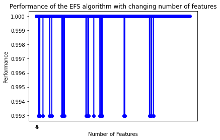
Import the mlxtend plotting utility and visualise how performance and its standard deviation change across all evaluated feature subset sizes:
from mlxtend.plotting import plot_sequential_feature_selection as plot_sfsNow, try to plot the graph of the performance with changing number of features.
plot_sfs(efs.get_metric_dict(), kind='std_dev')
plt.title('Performance of the EFS algorithm with changing number of features')
plt.show()
The chart below plots accuracy (y-axis) against number of features (x-axis) for all 2002 evaluated subsets. Most subsets cluster near perfect accuracy (1.0), with a few outliers near 0.993, confirming that the Wine dataset is highly separable when the right features are used:
Conclusion
In this tutorial you applied all three wrapper-based feature selection strategies to scikit-learn's Wine dataset using the mlxtend library. Sequential Forward Selection (SFS) identified that just 3 features — magnesium, flavanoids, and color_intensity — achieve 98.6 % cross-validated accuracy. Sequential Backward Selection (SBS) retained 8 features at the same peak score. Exhaustive Feature Selection (EFS) confirmed a perfect training accuracy with only 4 features (alcohol, malic_acid, ash, alcalinity_of_ash), though cv=None means that score reflects training data only.
Key takeaways:
- Wrapper methods use a real model's performance as the selection criterion, making them sensitive to feature interactions that filter methods miss.
- SFS and SBS are greedy and fast but not guaranteed to find the global optimum — they can get stuck at locally good subsets.
- EFS guarantees the globally optimal subset within the specified size range, but evaluation cost grows combinatorially with the number of features.
- Passing
k_featuresas a range tuple(min, max)letsSequentialFeatureSelectorautomatically return the subset size that maximised cross-validated performance within the search. - A perfect training score from EFS with
cv=Noneshould always be verified on a held-out test set before being trusted.
Next steps:
- Contrast wrapper methods with embedded regularization techniques in Lasso and Ridge Regularisation for Feature Selection, which select features as part of model training itself.
- Explore Recursive Feature Elimination (RFE) to see how tree-based and gradient-based estimators rank and prune features in one pass.
- Start from simpler statistical filtering in Feature Selection with Filter Methods to understand the baseline before moving to wrapper and embedded approaches.

