Speed Up Training with Bagging

Training a Support Vector Machine on a large dataset can be painfully slow. SVM time complexity scales as $O(n^3)$ with the number of samples $n$, so tripling your dataset size makes training 27 times slower. Bagging — short for Bootstrap Aggregating — sidesteps this by splitting the data into smaller subsets, training a separate model on each, and then combining their predictions. Because each model trains on a fraction of the data, the per-model cost drops dramatically.

In this tutorial you will use scikit-learn's BaggingClassifier to train ten parallel SVM estimators on the Iris dataset (scaled to 75,000 samples) and compare the result against a single SVM trained on the full dataset. You will see training time fall from 34.5 seconds to 10.5 seconds with no loss in accuracy.

Prerequisites: Python 3.x, NumPy, scikit-learn.

How Bagging Works

Bagging works by creating multiple bootstrap samples — random subsets drawn with replacement from your training data — and training an independent classifier on each one. The final prediction is produced by aggregating all classifiers, typically by majority vote for classification tasks.

The diagram below shows the full flow: a training dataset is split into three bootstrap sets, each subset trains its own classifier, and all three predictions are combined at the aggregation step to produce the final output $\hat{y}$:

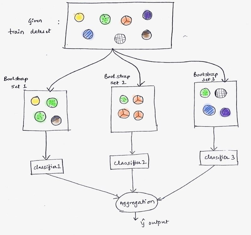
To understand why this matters, consider SVM time complexity:

For example, if 1,000 samples take 10 seconds to train, then 3,000 samples would take roughly $10\times 3^3=270$ seconds. But if you split those 3,000 samples into three sets of 1,000, each set takes 10 seconds — a total of 30 seconds instead of 270.

Loading the Iris Dataset

Start by importing the libraries you will use throughout this tutorial:

import numpy as np
from sklearn.ensemble import BaggingClassifier
from sklearn import datasets
from sklearn.svm import SVC

Load the Iris dataset and inspect its keys to confirm what fields are available:

iris = datasets.load_iris()
iris.keys()

dict_keys(['data', 'target', 'target_names', 'DESCR', 'feature_names', 'filename'])

Print the full dataset description to understand the feature layout and class distribution:

print(iris.DESCR)

.. _iris_dataset:

Iris plants dataset
--------------------

**Data Set Characteristics:**

    :Number of Instances: 150 (50 in each of three classes)
    :Number of Attributes: 4 numeric, predictive attributes and the class
    :Attribute Information:
        - sepal length in cm
        - sepal width in cm
        - petal length in cm
        - petal width in cm
        - class:
                - Iris-Setosa
                - Iris-Versicolour
                - Iris-Virginica

    :Summary Statistics:

    ============== ==== ==== ======= ===== ====================
                    Min  Max   Mean    SD   Class Correlation
    ============== ==== ==== ======= ===== ====================
    sepal length:   4.3  7.9   5.84   0.83    0.7826
    sepal width:    2.0  4.4   3.05   0.43   -0.4194
    petal length:   1.0  6.9   3.76   1.76    0.9490  (high!)
    petal width:    0.1  2.5   1.20   0.76    0.9565  (high!)
    ============== ==== ==== ======= ===== ====================

    :Missing Attribute Values: None
    :Class Distribution: 33.3% for each of 3 classes.
    :Creator: R.A. Fisher
    :Donor: Michael Marshall (MARSHALL%PLU@io.arc.nasa.gov)
    :Date: July, 1988

The famous Iris database, first used by Sir R.A. Fisher. The dataset is taken
from Fisher's paper. Note that it's the same as in R, but not as in the UCI
Machine Learning Repository, which has two wrong data points.

This is perhaps the best known database to be found in the
pattern recognition literature.  Fisher's paper is a classic in the field and
is referenced frequently to this day.  (See Duda & Hart, for example.)  The
data set contains 3 classes of 50 instances each, where each class refers to a
type of iris plant.  One class is linearly separable from the other 2; the
latter are NOT linearly separable from each other.

Extract the feature matrix X and the label vector y from the loaded dataset:

X = iris.data
y = iris.target

Check the shape of both arrays to confirm you have 150 samples with 4 features each:

X.shape, y.shape

((150, 4), (150,))

The Iris dataset has only 150 samples, which is too small to demonstrate a meaningful training-time difference. You will use np.repeat() to replicate the data 500 times, producing 75,000 samples that make the SVM cubic cost visible:

X = np.repeat(X, repeats=500, axis = 0)
y = np.repeat(y, repeats=500, axis = 0)

Confirm the expanded shape before training:

X.shape, y.shape

((75000, 4), (75000,))

Training Without Bagging

Train a single linear SVM on all 75,000 samples. The %%time magic cell records the wall-clock time so you have a baseline to compare against:

%%time
clf = SVC(kernel='linear', probability=True, class_weight='balanced')
clf.fit(X, y)
print('SVC: ', clf.score(X, y))

SVC:  0.98
Wall time: 34.5sec

The single SVM reaches 98 % accuracy but takes 34.5 seconds — a direct consequence of the cubic scaling discussed earlier.

Training With Bagging

Now wrap the same SVM in a BaggingClassifier. Setting n_estimators=10 creates ten sub-classifiers, and max_samples=1.0/n_estimators gives each one one-tenth of the full dataset (7,500 samples). Each estimator trains on a much smaller slice, so the cubic cost is applied to 7,500 samples rather than 75,000:

%%time
n_estimators = 10
clf = BaggingClassifier(SVC(kernel='linear', probability=True, class_weight='balanced'), n_estimators=n_estimators, max_samples=1.0/n_estimators)
clf.fit(X, y)
print('SVC: ', clf.score(X, y))

SVC:  0.98
Wall time: 10.5 s

The BaggingClassifier achieves the same 98 % accuracy in just 10.5 seconds — a 3.3× speedup with no trade-off in predictive performance.

Conclusion

In this tutorial you trained a linear SVM with and without bagging on a 75,000-sample version of the Iris dataset. The single SVM took 34.5 seconds to reach 98 % accuracy; the BaggingClassifier with ten estimators matched that accuracy in 10.5 seconds by splitting the data into smaller bootstrap subsets and training each estimator in parallel.

Key takeaways:

• SVM training time scales as $O(n^3)$, so bagging delivers its largest gains on large datasets where the cubic cost is most visible.
• BaggingClassifier wraps any scikit-learn estimator — you are not limited to SVMs.
• Setting max_samples=1.0/n_estimators ensures each sub-model sees a non-overlapping fraction of the data, maximising the speed benefit.
• Bagging can match or exceed single-model accuracy because aggregating diverse estimators reduces variance.

Next steps:

• Read Ensemble Learning for a broader look at bagging, boosting, and stacking in one place.
• Explore Random Forest to see how decision-tree bagging is extended into one of the most robust ensemble models available.
• Try replacing SVC with a DecisionTreeClassifier as the base estimator and compare how training time and accuracy change across different n_estimators values.