Dimensionality Reduction with LDA and PCA in Python

When a dataset has hundreds of features, training a model becomes slow and the risk of overfitting increases. Dimensionality reduction is the process of compressing a high-dimensional feature space into a smaller one while retaining as much useful information as possible. Two of the most widely used techniques are Principal Component Analysis (PCA) and Linear Discriminant Analysis (LDA).

In this tutorial you will apply both PCA and LDA to the Santander customer satisfaction dataset, which starts with 370 features. After cleaning the data you will use a Random Forest classifier to measure whether — and how much — compression hurts accuracy, and you will see that LDA can cut training time in half with only a small accuracy cost.

Prerequisites: Python 3.x, scikit-learn, pandas, NumPy, Matplotlib, seaborn.

What is LDA (Linear Discriminant Analysis)?

LDA — Linear Discriminant Analysis — is a supervised dimensionality reduction technique, meaning it uses the class labels in your data to guide the compression. The goal is to find a new axis (or set of axes) onto which you can project your data so that the different classes end up as far apart as possible.

To find that axis LDA solves two sub-problems simultaneously:

Maximise between-class distance — push the centroid of each class as far from the other centroids as possible.
Minimise within-class scatter — keep the data points inside each class tightly clustered around their centroid.

The scatter that LDA minimises is expressed as $s^{2}$ . Formally, LDA finds a projection vector $w$ that maximises the following ratio:

J (w) = \frac{w ^{T} S _{B} w}{w ^{T} S _{W} w}

Where:

$w$ — the projection vector (the new axis you are finding)
$S_{B}$ — the between-class scatter matrix (measures how far apart the class centroids are)
$S_{W}$ — the within-class scatter matrix (measures how spread out the samples are within each class)
$J (w)$ — the Fisher criterion; maximising it gives the best separating projection

One practical constraint: the maximum number of LDA components you can extract equals the number of classes minus one. For a binary classification problem (two classes, such as Santander's TARGET of 0 or 1) the maximum is 1 component.

What is PCA (Principal Component Analysis)?

PCA — Principal Component Analysis — is an unsupervised dimensionality reduction technique. It ignores class labels entirely and instead looks for the directions in your data that carry the most variance — the so-called principal components.

The diagram below shows PCA on a 2-D dataset. The left panel displays the original input data with the two principal component axes (eigenvectors) overlaid; the right panel shows the same data reprojected onto those two components:

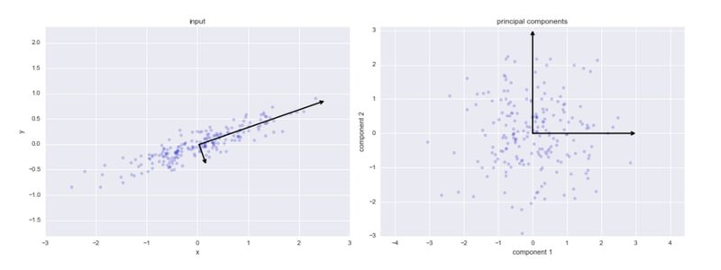
PCA diagram showing original data with eigenvector axes on the left, and the same data reprojected onto principal components on the right

The first principal component points in the direction of greatest variance; the second is orthogonal (perpendicular) to the first and captures the next greatest variance. PCA finds these components by performing an eigendecomposition of the covariance matrix. The key formula that describes how much variance component $k$ explains is:

Explained Variance Ratio_{k} = \frac{λ _{k}}{\sum _{i = 1}^{n} λ _{i}}

Where:

$λ_{k}$ — the eigenvalue of the $k$ -th principal component
$\sum_{i = 1}^{n} λ_{i}$ — the sum of all eigenvalues (total variance in the dataset)
$Explained Variance Ratio_{k}$ — the fraction of total variance captured by component $k$

When to Use PCA

Data visualisation: With hundreds of features it is impossible to plot your data meaningfully. PCA lets you compress it to 2 or 3 components so you can scatter-plot the samples and spot structure, clusters, or outliers.

Speeding up ML algorithms: Training time grows with the number of features. If your model is too slow, applying PCA first can dramatically shorten training and inference time without sacrificing much accuracy — as you will see in the benchmarks below.

Setting Up: Imports and Data Loading

Start by importing every library the tutorial needs. Keeping all imports in one block at the top makes dependencies explicit.

PYTHON

import pandas as pd
import numpy as np
import seaborn as sns
import matplotlib.pyplot as plt
%matplotlib inline

PYTHON

from sklearn.model_selection import train_test_split
from sklearn.ensemble import RandomForestClassifier
from sklearn.metrics import accuracy_score, roc_auc_score
from sklearn.feature_selection import VarianceThreshold
from sklearn.preprocessing import StandardScaler

Load the first 20 000 rows of the Santander dataset into a DataFrame:

PYTHON

data = pd.read_csv('santander.csv', nrows = 20000)
data.head()

Separate features from the target column and confirm the shapes:

PYTHON

X = data.drop('TARGET', axis = 1)
y = data['TARGET']
X.shape, y.shape

OUTPUT

((20000, 370), (20000,))

The dataset has 370 features. Split it into training (80 %) and test (20 %) sets, using stratify=y to preserve the class balance:

PYTHON

X_train, X_test, y_train, y_test = train_test_split(X, y, test_size = 0.2, random_state = 0, stratify = y)

Cleaning the Data Before Reduction

Before applying LDA or PCA, it is good practice to remove features that add noise but no signal. Three common culprits are constant features, quasi-constant features, and duplicate features.

Removing Constant and Quasi-Constant Features

A VarianceThreshold with threshold=0.01 removes any feature where 99 % or more of its values are identical. These features carry almost no information:

PYTHON

constant_filter = VarianceThreshold(threshold=0.01)
constant_filter.fit(X_train)
X_train_filter = constant_filter.transform(X_train)
X_test_filter = constant_filter.transform(X_test)
X_train_filter.shape, X_test_filter.shape

OUTPUT

((16000, 245), (4000, 245))

The filter cut the feature count from 370 down to 245.

Removing Duplicate Features

Duplicated columns are pure redundancy — they inflate training time without adding information. Transposing the matrix lets pandas detect duplicate rows (which are duplicate columns in the original):

PYTHON

X_train_T = X_train_filter.T
X_test_T = X_test_filter.T
X_train_T = pd.DataFrame(X_train_T)
X_test_T =pd.DataFrame(X_test_T)X_train_T.duplicated().sum()

OUTPUT

PYTHON

duplicated_features = X_train_T.duplicated()
features_to_keep = [not index for index in duplicated_features]
X_train_unique = X_train_T[features_to_keep].T
X_test_unique = X_test_T[features_to_keep].T

Standardise the surviving features so that all columns are on the same scale before computing distances or variances:

PYTHON

scaler = StandardScaler().fit(X_train_unique)
X_train_unique = scaler.transform(X_train_unique)
X_test_unique = scaler.transform(X_test_unique)
X_train_unique = pd.DataFrame(X_train_unique)
X_test_unique = pd.DataFrame(X_test_unique)X_train_unique.shape, X_test_unique.shape

OUTPUT

((16000, 227), (4000, 227))

Removing Correlated Features

Highly correlated features are near-duplicates in a statistical sense. The function below identifies every pair of features with absolute correlation above 0.70 and collects the columns to drop:

PYTHON

corrmat = X_train_unique.corr()

PYTHON

def get_correlation(data, threshold):
    corr_col = set()
    corrmat = data.corr()
    for i in range(len(corrmat.columns)):
        for j in range(i):
            if abs(corrmat.iloc[i, j]) > threshold:
                colname = corrmat.columns[i]
                corr_col.add(colname)
    return corr_col

corr_features = get_correlation(X_train_unique, 0.70)
print('correlated features: ', len(set(corr_features)) )

OUTPUT

correlated features:  148

PYTHON

X_train_uncorr = X_train_unique.drop(labels=corr_features, axis = 1)
X_test_uncorr = X_test_unique.drop(labels = corr_features, axis = 1)
X_train_uncorr.shape, X_test_uncorr.shape

OUTPUT

((16000, 79), (4000, 79))

After removing constant, duplicate, and correlated features, you are left with 79 features — down from 371. This is the cleaned dataset you will feed into LDA and PCA.

Dimensionality Reduction with LDA

Import LinearDiscriminantAnalysis from scikit-learn:

PYTHON

from sklearn.discriminant_analysis import LinearDiscriminantAnalysis as LDA

Because the Santander problem is binary (classes 0 and 1), the maximum number of LDA components is number of classes − 1 = 1. Passing n_components=1 is both correct and explicit:

PYTHON

lda = LDA(n_components=1)
X_train_lda = lda.fit_transform(X_train_uncorr, y_train)
X_test_lda = lda.transform(X_test_uncorr)

Check that the data has been compressed to a single column:

PYTHON

X_train_lda.shape, X_test_lda.shape

OUTPUT

((16000, 1), (4000, 1))

Define a helper function that trains a Random Forest and prints accuracy so you can reuse it across all comparisons:

PYTHON

def run_randomForest(X_train, X_test, y_train, y_test):
    clf = RandomForestClassifier(n_estimators=100, random_state=0, n_jobs=-1)
    clf.fit(X_train, y_train)
    y_pred = clf.predict(X_test)
    print('Accuracy on test set: ')
    print(accuracy_score(y_test, y_pred))

Benchmark the LDA-reduced dataset first:

PYTHON

%%time
run_randomForest(X_train_lda, X_test_lda, y_train, y_test)

OUTPUT

Accuracy on test set:
0.93025
CPU times: user 3.35 s, sys: 64.3 ms, total: 3.41 s
Wall time: 1.1 s

Now benchmark the 79-feature cleaned dataset (before LDA):

PYTHON

%%time
run_randomForest(X_train_uncorr, X_test_uncorr, y_train, y_test)

OUTPUT

Accuracy on test set:
0.9585
CPU times: user 3.41 s, sys: 82 ms, total: 3.49 s
Wall time: 1.2 s

Finally, benchmark on the original 370-feature dataset to see the full picture:

PYTHON

%%time
run_randomForest(X_train, X_test, y_train, y_test)

OUTPUT

Accuracy on test set:
0.9585
CPU times: user 6.68 s, sys: 143 ms, total: 6.83 s
Wall time: 2.01 s

The original dataset and the 79-feature cleaned version both achieve 95.85 % accuracy, but the original takes 2 seconds versus 1.2 seconds. The LDA-reduced dataset (1 feature) runs in 1.1 seconds but accuracy drops to 93.0 %. LDA does not guarantee it preserves predictive accuracy — it guarantees a dramatic reduction in dimensionality and training time. The accuracy trade-off is small here, and in production systems with millions of rows the speed gain would be far more significant.

Dimensionality Reduction with PCA

Import PCA from scikit-learn's decomposition module:

PYTHON

from sklearn.decomposition import PCA

Fit a PCA model that keeps 2 principal components. Unlike LDA, PCA is not constrained by the number of classes:

PYTHON

pca = PCA(n_components=2, random_state=42)
pca.fit(X_train_uncorr)
PCA(copy=True, iterated_power='auto', n_components=2, random_state=42, svd_solver='auto', tol=0.0, whiten=False)

Project both splits into the 2-component PCA space:

PYTHON

X_train_pca = pca.transform(X_train_uncorr)
X_test_pca = pca.transform(X_test_uncorr)
X_train_pca.shape, X_test_pca.shape

OUTPUT

((16000, 2), (4000, 2))

Benchmark the PCA-reduced dataset:

PYTHON

%%time
run_randomForest(X_train_pca, X_test_pca, y_train, y_test)

OUTPUT

Accuracy on test set:
0.956
CPU times: user 3.06 s, sys: 67.9 ms, total: 3.12 s
Wall time: 999 ms

Compare against the original dataset (re-run for a fair side-by-side):

PYTHON

%%time
run_randomForest(X_train, X_test, y_train, y_test)

OUTPUT

Accuracy on test set:
0.9585
CPU times: user 6.75 s, sys: 138 ms, total: 6.89 s
Wall time: 2.13 s

The 79-feature uncorrected dataset contains 79 features before PCA:

PYTHON

X_train_uncorr.shape

OUTPUT

(16000, 79)

How Accuracy Changes with Component Count

It is worth checking whether using more than 2 components improves accuracy. The loop below trains and evaluates a Random Forest for 1, 2, 3, and 4 PCA components:

PYTHON

for component in range(1,5):
    pca = PCA(n_components=component, random_state=42)
    pca.fit(X_train_uncorr)
    X_train_pca = pca.transform(X_train_uncorr)
    X_test_pca = pca.transform(X_test_uncorr)
    print('Selected Components: ', component)
    run_randomForest(X_train_pca, X_test_pca, y_train, y_test)
    print()

OUTPUT

Selected Components:  1
Accuracy on test set:
0.92375

Selected Components:  2
Accuracy on test set:
0.956

Selected Components:  3
Accuracy on test set:
0.95675

Selected Components:  4
Accuracy on test set:
0.95825

With just 2 components you already recover most of the accuracy achievable with 79 features (95.6 % vs 95.85 %), and adding a third or fourth component brings only marginal gains. This demonstrates the power of PCA: a handful of components can often replace dozens of raw features.

Conclusion

In this tutorial you cleaned the Santander dataset from 370 features down to 79 by removing constant, duplicate, and highly correlated columns. You then compressed those 79 features further using both LDA (to 1 component) and PCA (to 2 components) and benchmarked a Random Forest classifier across all three versions.

Key takeaways:

LDA is supervised — it uses class labels to find a projection that maximises separation between classes. Because it is constrained to n_classes − 1 components, it is most powerful for multi-class problems.
PCA is unsupervised — it finds the directions of maximum variance regardless of labels. Even 2 PCA components can retain 95.6 % of the original accuracy on this dataset.
Both techniques roughly halved training time compared to the raw 370-feature dataset, with less than 3 percentage points of accuracy loss.
Always clean your data (remove constant, duplicate, and correlated features) before applying dimensionality reduction — the algorithms work better on a lean, high-quality feature set.
Neither LDA nor PCA guarantees higher accuracy; they guarantee a smaller, faster representation. Use them when speed or visualisation matters more than squeezing out the last fraction of a percent.

Next steps:

Deepen your understanding of how PCA fits into a full machine learning pipeline by reading PCA with Python — Principal Component Analysis.
Explore earlier stages of the feature engineering workflow in Feature Selection with Filtering Methods, which covers constant, quasi-constant, and duplicate removal in detail.
Learn how Random Forest makes use of reduced feature spaces, and compare it with SVM — a classifier that benefits especially from compact, well-separated feature representations.

Dimensionality Reduction with LDA and PCA in Python

Topics You Will Master

What is LDA (Linear Discriminant Analysis)?

What is PCA (Principal Component Analysis)?

When to Use PCA

Setting Up: Imports and Data Loading

Cleaning the Data Before Reduction

Removing Constant and Quasi-Constant Features

Removing Duplicate Features

Removing Correlated Features

Dimensionality Reduction with LDA

Dimensionality Reduction with PCA

How Accuracy Changes with Component Count

Conclusion

Latest recommendations you might like

LinkedIn Auto Connect Bot

Feature Selection with Mutual Information

Find this tutorial useful?

Discussion & Comments