
Choosing which features to keep is one of the most impactful decisions in a machine learning project. Including too many features slows training, increases overfitting risk, and makes models harder to interpret. Mutual information is a filter-based method that scores each feature by how much information it shares with the target variable — before any model is trained.
Mutual information (MI) measures statistical dependence between two variables. Unlike Pearson correlation, which only captures straight-line (linear) relationships, mutual information can detect any kind of relationship — linear or not. A score of 0 means the feature and the target are completely independent; a higher score means the feature carries more information about the target.
The formal definition of mutual information between two random variables and is:
Where:
- — the mutual information score between variables and
- — the joint probability of and occurring together
- — the marginal probability of alone
- — the marginal probability of alone
When , the variables are independent and . The more their joint distribution diverges from independence, the larger becomes.
In this tutorial you will apply mutual information to a high-dimensional bank customer churn dataset (370 features) for a classification task and to the Boston Housing dataset (13 features) for a regression task. You will compare model accuracy and training speed before and after feature selection.
You can also
.Prerequisites: Python 3.x, Scikit-learn, Pandas, NumPy, Matplotlib, Seaborn.
Classification Problem
We will demonstrate mutual information feature selection on a classification dataset. The dataset is available at github.com/laxmimerit/Data-Files-for-Feature-Selection.
Import the required libraries for data manipulation, visualization, and modeling:
import numpy as np
import pandas as pd
import matplotlib.pyplot as plt
import seaborn as sns
Import Scikit-learn modules for modeling, metrics, and feature selection:
from sklearn.model_selection import train_test_split
from sklearn.ensemble import RandomForestClassifier
from sklearn.metrics import accuracy_scorefrom sklearn.feature_selection import VarianceThreshold, mutual_info_classif, mutual_info_regression
from sklearn.feature_selection import SelectKBest, SelectPercentileRead the first 20,000 rows of the dataset:
data = pd.read_csv('train.csv', nrows = 20000)
data.head()| ID | var3 | var15 | imp_ent_var16_ult1 | imp_op_var39_comer_ult1 | imp_op_var39_comer_ult3 | imp_op_var40_comer_ult1 | imp_op_var40_comer_ult3 | imp_op_var40_efect_ult1 | imp_op_var40_efect_ult3 | ... | saldo_medio_var33_hace2 | saldo_medio_var33_hace3 | saldo_medio_var33_ult1 | saldo_medio_var33_ult3 | saldo_medio_var44_hace2 | saldo_medio_var44_hace3 | saldo_medio_var44_ult1 | saldo_medio_var44_ult3 | var38 | TARGET | |
|---|---|---|---|---|---|---|---|---|---|---|---|---|---|---|---|---|---|---|---|---|---|
| 0 | 1 | 2 | 23 | 0.0 | 0.0 | 0.0 | 0.0 | 0.0 | 0 | 0 | ... | 0.0 | 0.0 | 0.0 | 0.0 | 0.0 | 0.0 | 0.0 | 0.0 | 39205.170000 | 0 |
| 1 | 3 | 2 | 34 | 0.0 | 0.0 | 0.0 | 0.0 | 0.0 | 0 | 0 | ... | 0.0 | 0.0 | 0.0 | 0.0 | 0.0 | 0.0 | 0.0 | 0.0 | 49278.030000 | 0 |
| 2 | 4 | 2 | 23 | 0.0 | 0.0 | 0.0 | 0.0 | 0.0 | 0 | 0 | ... | 0.0 | 0.0 | 0.0 | 0.0 | 0.0 | 0.0 | 0.0 | 0.0 | 67333.770000 | 0 |
| 3 | 8 | 2 | 37 | 0.0 | 195.0 | 195.0 | 0.0 | 0.0 | 0 | 0 | ... | 0.0 | 0.0 | 0.0 | 0.0 | 0.0 | 0.0 | 0.0 | 0.0 | 64007.970000 | 0 |
| 4 | 10 | 2 | 37 | 0.0 | 0.0 | 0.0 | 0.0 | 0.0 | 0 | 0 | ... | 0.0 | 0.0 | 0.0 | 0.0 | 0.0 | 0.0 | 0.0 | 0.0 | 117310.979016 | 0 |
Separate the target variable and inspect the shape of the features:
X = data.drop('TARGET', axis = 1)
y = data['TARGET']
X.shape, y.shape((20000, 370), (20000,))The dataset contains 20,000 rows and 370 feature columns. Split it into training and testing sets, stratifying on the target to preserve class balance:
X_train, X_test, y_train, y_test = train_test_split(X, y, test_size = 0.2, random_state = 0, stratify = y)Remove Constant, Quasi-Constant, and Duplicate Features
Before calculating mutual information, it is important to remove features that carry no information at all. A constant feature has the same value for every row. A quasi-constant feature has almost the same value (for example, 99% of rows are zero). A duplicate feature is an exact copy of another column. None of these add predictive power, and keeping them wastes computation.
You can also
.Use VarianceThreshold with a threshold of 0.01 to remove quasi-constant features (those with less than 1% variance):
constant_filter = VarianceThreshold(threshold=0.01)
constant_filter.fit(X_train)
X_train_filter = constant_filter.transform(X_train)
X_test_filter = constant_filter.transform(X_test)
Transpose the filtered datasets so that each feature becomes a row, then wrap them in a DataFrame — this makes it easy to use duplicated() to spot identical features:
X_train_T = X_train_filter.T
X_test_T = X_test_filter.T
X_train_T = pd.DataFrame(X_train_T)
X_test_T = pd.DataFrame(X_test_T)
Count the number of duplicated rows (features) in the training dataset:
X_train_T.duplicated().sum()18There are 18 duplicate features. Identify them and keep only the unique ones:
duplicated_features = X_train_T.duplicated()features_to_keep = [not index for index in duplicated_features]
X_train_unique = X_train_T[features_to_keep].T
X_test_unique = X_test_T[features_to_keep].T
X_train_unique.shape, X_test_unique.shape((16000, 227), (4000, 227))After removing constant, quasi-constant, and duplicate features, the feature space drops from 370 to 227 columns. This is a clean input for mutual information scoring.
Calculate the Mutual Information
With the cleaned feature set, compute mutual information scores for all 227 features against the target using mutual_info_classif. This function estimates how much information each feature shares with the class label:
mi = mutual_info_classif(X_train_unique, y_train)
len(mi)227Inspect the first 10 mutual information scores to get a sense of the range:
mi[: 10]array([0.0025571 , 0. , 0.01479401, 0. , 0. ,
0.00133223, 0. , 0. , 0.00197431, 0. ])Several features score exactly 0, meaning they are statistically independent of the target. Convert the scores to a Pandas Series, align them with the column names, and sort in descending order:
mi = pd.Series(mi)
mi.index = X_train_unique.columnsmi.sort_values(ascending=False, inplace = True)The bar plot below shows that only a small number of features carry a high mutual information score — most features cluster near zero:
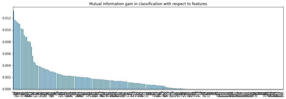
This long-tail distribution is typical: a handful of features drive most of the predictive signal. Use SelectPercentile to keep the top 10% of features automatically:
sel = SelectPercentile(mutual_info_classif, percentile=10).fit(X_train_unique, y_train)
X_train_unique.columns[sel.get_support()]Int64Index([ 2, 22, 40, 49, 50, 51, 52, 61, 86, 91, 98, 100, 101,
105, 119, 125, 127, 182, 187, 209, 210, 211, 212],
dtype='int64')Count the total number of features kept:
len(X_train_unique.columns[sel.get_support()])23The top 10% corresponds to 23 features. Transform both datasets to keep only these:
X_train_mi = sel.transform(X_train_unique)
X_test_mi = sel.transform(X_test_unique)
X_train_mi.shape(16000, 23)Build the Model and Compare Performance
To confirm that 23 features are enough, train a RandomForestClassifier on both the reduced set and the full original dataset, then compare accuracy and wall time.
Define a helper function that trains the classifier and prints accuracy:
def run_randomForest(X_train, X_test, y_train, y_test):
    clf = RandomForestClassifier(n_estimators=100, random_state=0, n_jobs=-1)
    clf.fit(X_train, y_train)
    y_pred = clf.predict(X_test)
    print('Accuracy on test set: ')
    print(accuracy_score(y_test, y_pred))
Train and evaluate the model using only the 23 mutual-information-selected features:
%%time
run_randomForest(X_train_mi, X_test_mi, y_train, y_test)Accuracy on test set:
0.95825
Wall time: 1.14 sTrain and evaluate the model using all 370 original features:
%%time
run_randomForest(X_train, X_test, y_train, y_test)Accuracy on test set:
0.9585
Wall time: 2.41 sCalculate the percentage decrease in training time when using the selected features:
(1.46-0.57)*100/1.4660.95890410958904The reduced model (23 features) scores 95.83% accuracy versus 95.85% for the full model — a negligible difference. Yet training time drops by approximately 61%. This is the core value of mutual information filtering: near-identical performance at a fraction of the computational cost.
Mutual Information for Regression
Mutual information also works for regression tasks where the target is a continuous number rather than a class label. mutual_info_regression estimates the information each feature shares with a continuous target. We will demonstrate this on the Boston Housing dataset.
Import the required libraries for regression datasets and metrics:
from sklearn.datasets import load_boston
from sklearn.linear_model import LinearRegression
from sklearn.metrics import mean_absolute_error, mean_squared_error, r2_score
Load the Boston housing dataset and print its description:
boston = load_boston()
print(boston.DESCR).. _boston_dataset:
Boston house prices dataset
---------------------------
**Data Set Characteristics:**
:Number of Instances: 506
:Number of Attributes: 13 numeric/categorical predictive. Median Value (attribute 14) is usually the target.
:Attribute Information (in order):
- CRIM per capita crime rate by town
- ZN proportion of residential land zoned for lots over 25,000 sq.ft.
- INDUS proportion of non-retail business acres per town
- CHAS Charles River dummy variable (= 1 if tract bounds river; 0 otherwise)
- NOX nitric oxides concentration (parts per 10 million)
- RM average number of rooms per dwelling
- AGE proportion of owner-occupied units built prior to 1940
- DIS weighted distances to five Boston employment centres
- RAD index of accessibility to radial highways
- TAX full-value property-tax rate per $10,000
- PTRATIO pupil-teacher ratio by town
- B 1000(Bk - 0.63)^2 where Bk is the proportion of blacks by town
- LSTAT % lower status of the population
- MEDV Median value of owner-occupied homes in $1000's
:Missing Attribute Values: None
:Creator: Harrison, D. and Rubinfeld, D.L.
This is a copy of UCI ML housing dataset.
https://archive.ics.uci.edu/ml/machine-learning-databases/housing/
This dataset was taken from the StatLib library which is maintained at Carnegie Mellon University.
The Boston house-price data of Harrison, D. and Rubinfeld, D.L. 'Hedonic
prices and the demand for clean air', J. Environ. Economics & Management,
vol.5, 81-102, 1978. Used in Belsley, Kuh & Welsch, 'Regression diagnostics
...', Wiley, 1980. N.B. Various transformations are used in the table on
pages 244-261 of the latter.
The Boston house-price data has been used in many machine learning papers that address regression
problems.Create a Pandas DataFrame from the features:
X = pd.DataFrame(data = boston.data, columns=boston.feature_names)
X.head()| CRIM | ZN | INDUS | CHAS | NOX | RM | AGE | DIS | RAD | TAX | PTRATIO | B | LSTAT | |
|---|---|---|---|---|---|---|---|---|---|---|---|---|---|
| 0 | 0.00632 | 18.0 | 2.31 | 0.0 | 0.538 | 6.575 | 65.2 | 4.0900 | 1.0 | 296.0 | 15.3 | 396.90 | 4.98 |
| 1 | 0.02731 | 0.0 | 7.07 | 0.0 | 0.469 | 6.421 | 78.9 | 4.9671 | 2.0 | 242.0 | 17.8 | 396.90 | 9.14 |
| 2 | 0.02729 | 0.0 | 7.07 | 0.0 | 0.469 | 7.185 | 61.1 | 4.9671 | 2.0 | 242.0 | 17.8 | 392.83 | 4.03 |
| 3 | 0.03237 | 0.0 | 2.18 | 0.0 | 0.458 | 6.998 | 45.8 | 6.0622 | 3.0 | 222.0 | 18.7 | 394.63 | 2.94 |
| 4 | 0.06905 | 0.0 | 2.18 | 0.0 | 0.458 | 7.147 | 54.2 | 6.0622 | 3.0 | 222.0 | 18.7 | 396.90 | 5.33 |
Assign the target variable (median home value) and split into training and test sets:
y = boston.targetX_train, X_test, y_train, y_test = train_test_split(X, y, test_size = 0.2, random_state = 0)Ranking Features by Mutual Information
Calculate mutual information scores for each of the 13 features against the continuous target, then sort them from most informative to least:
mi = mutual_info_regression(X_train, y_train)
mi = pd.Series(mi)
mi.index = X_train.columns
mi.sort_values(ascending=False, inplace = True)
miLSTAT 0.676729
RM 0.557777
INDUS 0.504754
PTRATIO 0.492141
NOX 0.445376
TAX 0.373128
CRIM 0.349371
AGE 0.347299
DIS 0.321057
RAD 0.203106
ZN 0.201467
B 0.152778
CHAS 0.008383
dtype: float64LSTAT (percentage of lower-status population) and RM (average rooms per dwelling) lead by a wide margin, while CHAS (a river-adjacency dummy variable) scores nearly zero. The bar plot below makes this ranking easy to read at a glance:
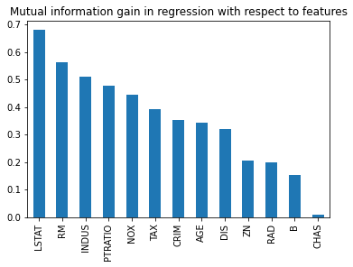
Selecting the Top Features
Use SelectKBest with k=9 to keep the nine most informative features:
sel = SelectKBest(mutual_info_regression, k = 9).fit(X_train, y_train)
X_train.columns[sel.get_support()]Index(['CRIM', 'INDUS', 'NOX', 'RM', 'AGE', 'DIS', 'TAX', 'PTRATIO', 'LSTAT'], dtype='object')Comparing Full vs. Reduced Feature Set
Fit a linear regression model on the full 13-feature dataset and compute the score — a measure of how much variance in the target the model explains (1.0 is perfect):
model = LinearRegression()
model.fit(X_train, y_train)
y_predict = model.predict(X_test)
r2_score(y_test, y_predict)0.5892223849182507Calculate the Root Mean Squared Error (RMSE) for the full-feature model. RMSE is in the same units as the target (thousands of dollars), so lower is better:
np.sqrt(mean_squared_error(y_test, y_predict))5.783509315085146For context, check the standard deviation of the target variable to understand the scale of the error:
np.std(y)9.188011545278203The RMSE of 5.78 is well below the target standard deviation of 9.19, which is a reasonable result for a simple linear model. Now transform the datasets to keep only the 9 selected features and repeat the evaluation:
X_train_9 = sel.transform(X_train)
X_train_9.shape(404, 9)X_test_9 = sel.transform(X_test)
model = LinearRegression()
model.fit(X_train_9, y_train)
y_predict = model.predict(X_test_9)
print('r2_score')
r2_score(y_test, y_predict)
r2_score0.5317127606961576Calculate the RMSE on the reduced dataset:
print('rmse')
np.sqrt(mean_squared_error(y_test, y_predict))rmse
6.175103151293747The 9-feature model yields an of 0.53 versus 0.59 for the full 13-feature model — a modest drop. For a dataset with only 13 features to begin with, the trade-off is less dramatic than in the classification example, but SelectKBest still removes the two weakest features (B and CHAS) cleanly and without model training.
Conclusion
In this tutorial you applied mutual information as a filter-based feature selection method to both a classification task (370 features, churn dataset) and a regression task (13 features, Boston Housing). By measuring the entropy shared between each feature and the target, you ranked all features without training any model, then selected the most informative subset using SelectPercentile and SelectKBest.
Key takeaways:
- Mutual information captures both linear and non-linear relationships, making it more powerful than simple correlation for feature ranking.
- In the classification experiment, keeping only 23 out of 370 features cut training time by 61% with no meaningful drop in accuracy (95.83% vs 95.85%).
mutual_info_classifis used for discrete targets;mutual_info_regressionis used for continuous targets — the selection API (SelectKBest,SelectPercentile) is identical for both.- Always remove constant, quasi-constant, and duplicate features before computing MI scores — they inflate the feature count without contributing information.
- MI is a greedy filter method: it evaluates features independently and does not account for interactions between features.
Next steps:
- Learn the preprocessing steps that precede mutual information scoring in Constant, Quasi-Constant, and Duplicate Feature Removal.
- Compare mutual information to chi-squared and Fisher scores in Feature Selection Using Fisher Score and Chi-Squared Test.
- Explore wrapper-based methods that consider feature interactions in Step Forward, Step Backward, and Exhaustive Feature Selection.

