
When you build a classification model, not every feature in your dataset is useful. Some features are statistically independent of the target variable — they carry no signal — and including them adds noise, slows training, and can hurt accuracy. Feature selection is the process of identifying and keeping only the features that matter.
For categorical features, the Chi-Squared () test is one of the most reliable filter methods. It is a statistical test that measures whether two categorical variables are independent of each other. A low p-value (a measure of statistical significance — closer to zero means stronger evidence against independence) tells you that a feature is likely related to the target class and worth keeping. A high p-value suggests the feature and target are independent, making the feature a good candidate for removal.
Fisher Score is a related supervised method that ranks each feature individually by how well it separates the classes — features that produce tight within-class clusters and wide between-class distances receive a higher score.
In this tutorial, you will apply both methods to the Titanic dataset to select the most informative categorical features, then validate those rankings by training Random Forest classifiers on progressively larger feature subsets.
You can also
.The Chi-Square test statistic is defined as:
Where:
- — the Chi-Squared test statistic; larger values indicate stronger dependence between the feature and the target
- — the observed frequency count for category in the data
- — the expected frequency count for category under the null hypothesis that the feature and target are independent
Prerequisites: Python 3.x, Scikit-learn, Pandas, NumPy, Seaborn, Matplotlib.
Loading the Required Dataset
Import all the libraries needed for data analysis, modeling, and statistical testing up front:
import numpy as np
import pandas as pd
import seaborn as sns
import matplotlib.pyplot as plt
%matplotlib inlinefrom sklearn.model_selection import train_test_split
from sklearn.ensemble import RandomForestClassifier
from sklearn.feature_selection import chi2
from sklearn.feature_selection import SelectKBest, SelectPercentile
from sklearn.metrics import accuracy_scoreLoad the Titanic dataset directly from Seaborn's built-in datasets:
titanic = sns.load_dataset('titanic')
titanic.head()| survived | pclass | sex | age | sibsp | parch | fare | embarked | class | who | adult_male | deck | embark_town | alive | alone | |
|---|---|---|---|---|---|---|---|---|---|---|---|---|---|---|---|
| 0 | 0 | 3 | male | 22.0 | 1 | 0 | 7.2500 | S | Third | man | True | NaN | Southampton | no | False |
| 1 | 1 | 1 | female | 38.0 | 1 | 0 | 71.2833 | C | First | woman | False | C | Cherbourg | yes | False |
| 2 | 1 | 3 | female | 26.0 | 0 | 0 | 7.9250 | S | Third | woman | False | NaN | Southampton | yes | True |
| 3 | 1 | 1 | female | 35.0 | 1 | 0 | 53.1000 | S | First | woman | False | C | Southampton | yes | False |
| 4 | 0 | 3 | male | 35.0 | 0 | 0 | 8.0500 | S | Third | man | True | NaN | Southampton | no | True |
Inspect the dataset for missing values so you know which columns need cleaning before modeling:
titanic.isnull().sum()survived 0
pclass 0
sex 0
age 177
sibsp 0
parch 0
fare 0
embarked 2
class 0
who 0
adult_male 0
deck 688
embark_town 2
alive 0
alone 0
dtype: int64The age column is missing 177 values and deck is missing 688 out of 891 — too many to impute reliably. Drop both columns, then drop any remaining rows with NaN values:
titanic.drop(labels = ['age', 'deck'], axis = 1, inplace = True)
titanic = titanic.dropna()
titanic.isnull().sum()survived 0
pclass 0
sex 0
sibsp 0
parch 0
fare 0
embarked 0
class 0
who 0
adult_male 0
embark_town 0
alive 0
alone 0
dtype: int64The Chi-Square test operates only on categorical (or discrete non-negative integer) features, so filter the dataset down to those columns only:
data = titanic[['pclass', 'sex', 'sibsp', 'parch', 'embarked', 'who', 'alone']].copy()
data.head()| pclass | sex | sibsp | parch | embarked | who | alone | |
|---|---|---|---|---|---|---|---|
| 0 | 3 | male | 1 | 0 | S | man | False |
| 1 | 1 | female | 1 | 0 | C | woman | False |
| 2 | 3 | female | 0 | 0 | S | woman | True |
| 3 | 1 | female | 1 | 0 | S | woman | False |
| 4 | 3 | male | 0 | 0 | S | man | True |
Confirm there are no missing values in your filtered feature set:
data.isnull().sum()pclass 0
sex 0
sibsp 0
parch 0
embarked 0
who 0
alone 0
dtype: int64Encoding Categorical Features
Scikit-learn's chi2 function requires non-negative integer inputs, so string and boolean columns must be mapped to numeric codes. Encode sex as 0 for male and 1 for female:
sex = {'male': 0, 'female': 1}
data['sex'] = data['sex'].map(sex)
data.head()| pclass | sex | sibsp | parch | embarked | who | alone | |
|---|---|---|---|---|---|---|---|
| 0 | 3 | 0 | 1 | 0 | S | man | False |
| 1 | 1 | 1 | 1 | 0 | C | woman | False |
| 2 | 3 | 1 | 0 | 0 | S | woman | True |
| 3 | 1 | 1 | 1 | 0 | S | woman | False |
| 4 | 3 | 0 | 0 | 0 | S | man | True |
Encode embarked port codes to integers, who passenger categories, and the boolean alone flag:
ports = {'S': 0, 'C': 1, 'Q': 2}
data['embarked'] = data['embarked'].map(ports)who = {'man': 0, 'woman': 1, 'child': 2}
data['who'] = data['who'].map(who)alone = {True: 1, False: 0}
data['alone'] = data['alone'].map(alone)
data.head()| pclass | sex | sibsp | parch | embarked | who | alone | |
|---|---|---|---|---|---|---|---|
| 0 | 3 | 0 | 1 | 0 | 0 | 0 | 0 |
| 1 | 1 | 1 | 1 | 0 | 1 | 1 | 0 |
| 2 | 3 | 1 | 0 | 0 | 0 | 1 | 1 |
| 3 | 1 | 1 | 1 | 0 | 0 | 1 | 0 |
| 4 | 3 | 0 | 0 | 0 | 0 | 0 | 1 |
Running the Chi-Squared Test
Separate your encoded features from the survival target, then check shapes to confirm alignment:
X = data.copy()
y = titanic['survived']
X.shape, y.shape((889, 7), (889,))Split into training and test sets (80 / 20), then call chi2 on the training data to compute the test statistic and p-value for each feature:
X_train, X_test, y_train, y_test = train_test_split(X, y, test_size = 0.2, random_state = 0)
f_score = chi2(X_train, y_train)
f_score(array([ 22.65169202, 152.91534343, 0.52934285, 10.35663782, 16.13255653, 161.42431175, 13.4382363 ]), array([1.94189138e-06, 3.99737147e-35, 4.66883271e-01, 1.29009955e-03, 5.90599986e-05, 5.52664700e-37, 2.46547298e-04]))chi2 returns a tuple: the first array contains the statistics and the second contains the corresponding p-values. Align the p-values with their feature names and sort them in ascending order so the most significant features appear first:
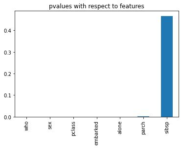
p_values = pd.Series(f_score[1], index = X_train.columns)
p_values.sort_values(ascending = True, inplace = True)
p_valueswho 5.526647e-37
sex 3.997371e-35
pclass 1.941891e-06
embarked 5.906000e-05
alone 2.465473e-04
parch 1.290100e-03
sibsp 4.668833e-01
dtype: float64who and sex have p-values near zero — extremely strong evidence of dependence on survival. sibsp has a p-value of 0.47, which is not statistically significant; it is effectively independent of survival and should be removed.
The bar chart below confirms this visually — all features except sibsp have p-values indistinguishable from zero, while sibsp stands clearly apart near 0.46:
Evaluating Feature Subsets with a Random Forest Classifier
To confirm that the statistical rankings translate into real accuracy gains, you will train a Random Forest classifier — an ensemble of decision trees that votes on the final prediction — on progressively larger subsets of features, ordered by their p-values from lowest to highest.
Define a helper function that fits a 100-tree Random Forest and prints the test accuracy:
def run_randomForest(X_train, X_test, y_train, y_test):
    clf = RandomForestClassifier(n_estimators=100, random_state=0, n_jobs=-1)
    clf.fit(X_train, y_train)
    y_pred = clf.predict(X_test)
    print('Accuracy: ', accuracy_score(y_test, y_pred))
Two Features: who and sex
Start with only the two most significant features to establish a baseline:
X_train_2 = X_train[['who', 'sex']]
X_test_2 = X_test[['who', 'sex']]%%time
run_randomForest(X_train_2, X_test_2, y_train, y_test)Accuracy: 0.7191011235955056
Wall time: 687 msWith just two features the model reaches 71.9% accuracy — a reasonable starting point given the limited information.
Three Features: who, sex, and pclass
Add pclass (the third most significant feature by p-value) and retrain:
X_train_3 = X_train[['who', 'sex', 'pclass']]
X_test_3 = X_test[['who', 'sex', 'pclass']]%%time
run_randomForest(X_train_3, X_test_3, y_train, y_test)Accuracy: 0.7415730337078652
Wall time: 649 msAdding pclass lifts accuracy to 74.2%, confirming that passenger class carries meaningful signal beyond what who and sex already capture.
Four Features: who, sex, pclass, and embarked
X_train_4 = X_train[['who', 'sex', 'pclass', 'embarked']]
X_test_4 = X_test[['who', 'sex', 'pclass', 'embarked']]%%time
run_randomForest(X_train_4, X_test_4, y_train, y_test)Accuracy: 0.7584269662921348
Wall time: 609 msThis is the best result so far at 75.8%. Including the embarkation port further improves the model.
Four Features: who, sex, pclass, and alone
Test whether swapping embarked for alone (the fifth-ranked feature) produces a different outcome:
X_train_4 = X_train[['who', 'sex', 'pclass', 'alone']]
X_test_4 = X_test[['who', 'sex', 'pclass', 'alone']]%%time
run_randomForest(X_train_4, X_test_4, y_train, y_test)Accuracy: 0.7528089887640449
Wall time: 710 msThe alone variant scores 75.3%, slightly below embarked — confirming that embarked carries marginally more survival signal at this subset size.
Five Features: who, sex, pclass, embarked, and alone
X_train_5 = X_train[['who', 'sex', 'pclass', 'embarked', 'alone']]
X_test_5 = X_test[['who', 'sex', 'pclass', 'embarked', 'alone']]%%time
run_randomForest(X_train_5, X_test_5, y_train, y_test)Accuracy: 0.7528089887640449
Wall time: 413 msAdding alone to the four-feature set provides no further gain — accuracy stays at 75.3%. This is a sign of diminishing returns as you approach the low-signal features.
Full Dataset: All Seven Features
Finally, evaluate using the complete set, including the statistically non-significant sibsp:
%%time
run_randomForest(X_train, X_test, y_train, y_test)Accuracy: 0.7359550561797753
Wall time: 576 msUsing all seven features drops accuracy back to 73.6%. The non-significant sibsp feature introduces noise that hurts generalization — a clear demonstration that more features does not always mean a better model.
Conclusion
In this tutorial, you applied the Chi-Squared () test to rank categorical features by their statistical dependence on survival in the Titanic dataset. Features like who, sex, and pclass showed p-values near zero — extremely strong evidence of a real relationship with the target. The statistically non-significant feature sibsp (p-value ≈ 0.47) was correctly identified as noise. A systematic experiment with Random Forest classifiers confirmed the rankings: four carefully chosen features (who, sex, pclass, embarked) achieved 75.8% accuracy, while using all seven features dropped accuracy to 73.6%.
Key takeaways:
- The Chi-Squared test quantifies independence between a categorical feature and the target class. A p-value below 0.05 is the conventional threshold for statistical significance.
- Fisher Score and both evaluate features individually — they find the best single features, not necessarily the best subset. Treat their rankings as a strong starting point, not a definitive answer.
- Encoding categorical features as non-negative integers is a prerequisite for
chi2; the function will raise an error on string or boolean inputs. - Removing a statistically insignificant feature can raise model accuracy — noise reduction often matters more than marginal information gain.
Next steps:
- Extend your feature selection knowledge to continuous numerical variables with Feature Selection Using Univariate ANOVA Test.
- Learn information-theory-based selection in Feature Selection Based on Mutual Information.
- Explore filter methods that remove constant, quasi-constant, and duplicate features first in Filtering Method: Constant, Quasi-Constant, and Duplicate Feature Removal.

