
When you build a classifier on a dataset with hundreds of features, many of those features are simply noise — they have no meaningful relationship with the target class. Training on noisy features wastes time and often hurts accuracy. Feature selection is the process of identifying and keeping only the features that actually carry predictive signal.
ANOVA (Analysis of Variance) is a classical statistics technique for testing whether the mean of a numeric variable differs significantly across two or more groups. In a classification context, the "groups" are the target classes, and you run one ANOVA test per feature. Features whose means differ significantly between classes get a high F-score and a low p-value — those are the features worth keeping.
In this tutorial you will apply ANOVA-based univariate feature selection to a real bank dataset with 370 features. You will remove constant and duplicate features first, then rank the remaining features by p-value, keep only those with , and compare a Random Forest trained on the full feature set against one trained on the reduced set.
Prerequisites: Python 3.x, Scikit-learn, Pandas, NumPy, Matplotlib, Seaborn.
The ANOVA F-Test Explained
Before writing any code, it helps to understand what ANOVA is actually computing.
The diagram below contrasts a t-test — which compares the means of exactly two groups — with ANOVA, which generalises that comparison to three or more groups:
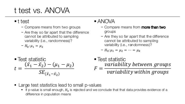
A t-test and ANOVA ask the same question — "are these group means farther apart than random sampling variability would explain?" — but ANOVA does it simultaneously for any number of groups. Both methods use the same underlying logic: if the spread between groups is large relative to the spread within groups, the difference is probably real.
The core ANOVA statistic is the F-ratio, defined as:
More precisely, each term is a mean square — a sum of squared deviations divided by its degrees of freedom:
Where:
- — the F-test statistic; larger values indicate stronger group separation
- — mean square between groups (between-class variance)
- — mean square within groups (within-class variance, also called residual error)
- — sum of squared deviations of group means from the overall mean
- — sum of squared deviations of individual values from their group mean
- — number of groups (classes)
- — total number of samples across all groups
A large means the feature separates the classes well. Scikit-learn converts each F-score into a p-value — the probability of observing that F-score (or higher) if the feature were actually uninformative. Features with are retained; everything else is dropped.
You can also
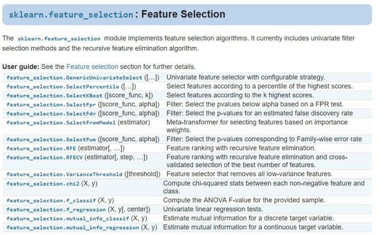
.Scikit-learn bundles all major univariate filter methods inside one module. The screenshot below shows the full list of classes available — including SelectKBest, f_classif, and VarianceThreshold, all of which you will use in this tutorial:
Classification Problem
Import the required libraries for data manipulation, plotting, and analysis:
import numpy as np
import pandas as pd
import matplotlib.pyplot as plt
import seaborn as sns
Import Scikit-learn modules for splitting data, building models, and calculating ANOVA statistics:
from sklearn.model_selection import train_test_split
from sklearn.ensemble import RandomForestClassifier
from sklearn.metrics import accuracy_score
from sklearn.feature_selection import VarianceThreshold
from sklearn.feature_selection import f_classif, f_regression
from sklearn.feature_selection import SelectKBest, SelectPercentile
The dataset used here is a bank customer satisfaction dataset with 370 numerical features and a binary TARGET column. You can download it from laxmimerit/Data-Files-for-Feature-Selection.
Load the first 20,000 rows of the classification dataset:
data = pd.read_csv('train.csv', nrows = 20000)
data.head()| ID | var3 | var15 | imp_ent_var16_ult1 | imp_op_var39_comer_ult1 | imp_op_var39_comer_ult3 | imp_op_var40_comer_ult1 | imp_op_var40_comer_ult3 | imp_op_var40_efect_ult1 | imp_op_var40_efect_ult3 | ... | saldo_medio_var33_hace2 | saldo_medio_var33_hace3 | saldo_medio_var33_ult1 | saldo_medio_var33_ult3 | saldo_medio_var44_hace2 | saldo_medio_var44_hace3 | saldo_medio_var44_ult1 | saldo_medio_var44_ult3 | var38 | TARGET | |
|---|---|---|---|---|---|---|---|---|---|---|---|---|---|---|---|---|---|---|---|---|---|
| 0 | 1 | 2 | 23 | 0.0 | 0.0 | 0.0 | 0.0 | 0.0 | 0 | 0 | ... | 0.0 | 0.0 | 0.0 | 0.0 | 0.0 | 0.0 | 0.0 | 0.0 | 39205.170000 | 0 |
| 1 | 3 | 2 | 34 | 0.0 | 0.0 | 0.0 | 0.0 | 0.0 | 0 | 0 | ... | 0.0 | 0.0 | 0.0 | 0.0 | 0.0 | 0.0 | 0.0 | 0.0 | 49278.030000 | 0 |
| 2 | 4 | 2 | 23 | 0.0 | 0.0 | 0.0 | 0.0 | 0.0 | 0 | 0 | ... | 0.0 | 0.0 | 0.0 | 0.0 | 0.0 | 0.0 | 0.0 | 0.0 | 67333.770000 | 0 |
| 3 | 8 | 2 | 37 | 0.0 | 195.0 | 195.0 | 0.0 | 0.0 | 0 | 0 | ... | 0.0 | 0.0 | 0.0 | 0.0 | 0.0 | 0.0 | 0.0 | 0.0 | 64007.970000 | 0 |
| 4 | 10 | 2 | 39 | 0.0 | 0.0 | 0.0 | 0.0 | 0.0 | 0 | 0 | ... | 0.0 | 0.0 | 0.0 | 0.0 | 0.0 | 0.0 | 0.0 | 0.0 | 117310.979016 | 0 |
Separate the features and target variable:
X = data.drop('TARGET', axis = 1)
y = data['TARGET']
X.shape, y.shape((20000, 370), (20000,))Split the data into training and test sets, stratifying on target classes to preserve the class ratio in both splits:
X_train, X_test, y_train, y_test = train_test_split(X, y, test_size = 0.2, random_state = 0, stratify = y)Remove Constant, Quasi-Constant, and Duplicate Features
Before running ANOVA, you should remove features that carry no information at all. Constant features take the same value for every sample; quasi-constant features take one value for more than 99% of samples. Neither can distinguish between classes.
You can also
.Initialize VarianceThreshold with a threshold of 0.01 (1% variance) to drop constant and quasi-constant columns:
constant_filter = VarianceThreshold(threshold=0.01)
constant_filter.fit(X_train)
X_train_filter = constant_filter.transform(X_train)
X_test_filter = constant_filter.transform(X_test)
Observe the remaining dimensions after thresholding:
X_train_filter.shape, X_test_filter.shape((16000, 245), (4000, 245))The variance filter reduced the feature count from 370 to 245. Next, remove duplicate features — columns that have identical values and therefore add no new information. For more details on this step, see Constant, Quasi-Constant, and Duplicate Feature Removal.
Transposing the data turns columns into rows, which lets Pandas identify duplicates efficiently:
X_train_T = X_train_filter.T
X_test_T = X_test_filter.TX_train_T = pd.DataFrame(X_train_T)
X_test_T = pd.DataFrame(X_test_T)Calculate the number of duplicate features in the dataset:
X_train_T.duplicated().sum()18There are 18 exact duplicate columns. Identify which rows (original columns) are duplicates:
duplicated_features = X_train_T.duplicated()Extract the unique features and transpose them back to the original orientation:
features_to_keep = [not index for index in duplicated_features]
X_train_unique = X_train_T[features_to_keep].T
X_test_unique = X_test_T[features_to_keep].TX_train_unique.shape, X_train.shape((16000, 227), (16000, 370))After removing constants and duplicates, the feature set shrank from 370 to 227 columns, with no loss of unique information.
Do the ANOVA F-Test
With clean, unique features in hand, you can now run the ANOVA test. f_classif returns two arrays: the F-score for each feature and the corresponding p-value. A high F-score (and therefore low p-value) means the feature's mean differs significantly between the two target classes.
Perform the univariate ANOVA F-test on the unique features:
sel = f_classif(X_train_unique, y_train)
sel(array([3.42911520e-01, 1.22929093e+00, 1.61291330e+02, 4.01025132e-01, 8.37661151e-01, 2.39279390e-03, 4.41633351e-02, 1.36337510e-01, 1.84647123e+00, 2.03640367e+00, 7.98057954e-03, 1.14063993e+00, 6.32266614e-03, 1.55626237e+01, 1.53553790e+01, 1.28615978e+01, 1.61834746e+01, 1.59638013e+01, 1.21977511e+01, 9.03776687e-02, 1.00443179e+00, 1.53946148e+01, 2.50428951e+02, 2.98696944e+01, 1.06266841e+01, 2.63630437e+01, 1.66417611e+01, 3.13699473e+01, 2.47256550e+01, 2.60021376e+01, 3.26742018e+01, 9.94259060e+00, 1.48208220e+01, 1.50040146e+01, 1.34739830e+01, 7.03118653e+00, 1.36234772e+01, 7.95962134e+00, 3.15161070e+02, 1.79631284e+00, 1.66910747e+00, 1.21138302e+01, 1.10928892e+01, 1.00443179e+00, 2.31851572e+00, 8.93973153e+01, 7.53868668e+00, 2.38490562e+02, 2.98696944e+01, 1.06266841e+01, 2.61694409e+01, 1.66053267e+01, 2.93013259e+01, 2.44433356e+01, 2.60021376e+01, 5.59623841e+00, 5.65080530e+00, 3.11715028e+01, 9.94259060e+00, 6.69237272e-01, 6.73931889e-01, 5.91355150e-01, 2.16653744e+00, 1.57036464e+00, 1.48180592e+01, 1.50040146e+01, 4.10147572e+00, 5.08119829e+00, 2.66061739e-01, 4.74076524e-04, 3.22895933e-02, 3.61497992e+00, 2.62641383e-01, 1.44465136e+00, 2.39577575e+00, 3.25151692e+00, 2.66120176e-01, 1.33584657e+00, 2.15986976e+00, 2.95680783e+01, 2.74320562e+02, 1.79136749e+00, 1.65942415e+00, 4.55732338e-01, 8.03423196e+01, 5.33753163e+00, 3.43569515e+00, 5.38991827e+00, 6.48705021e+00, 1.14907051e+01, 2.46676043e+02, 1.48964854e+00, 1.48528608e+00, 1.35499717e+00, 5.04105291e+00, 8.00857735e-02, 5.92081628e-01, 7.49538059e+00, 1.43768803e+01, 3.96797511e+00, 1.84630418e+01, 5.93034025e-01, 6.23117305e-02, 1.32846978e-01, 7.36058444e+00, 4.67453255e-01, 6.53434886e-01, 2.32603599e+01, 8.82160365e-02, 4.03681937e-01, 1.12281656e-01, 1.22229167e+00, 9.50849020e+00, 3.31504999e-01, 1.52799424e+02, 9.58201843e-01, 3.81283407e-01, 8.05456673e-01, 2.11768899e-01, 4.23427422e-02, 4.23427422e-02, 4.23427422e-02, 4.23675848e-01, 9.58201843e-01, 8.05456673e-01, 4.23675848e-01, 7.83475034e+00, 7.84514734e-01, 4.28901812e-02, 1.44260945e-01, 4.33508271e-02, 4.23427422e-02, 3.34880062e-02, 1.90957786e-01, 4.06328805e-01, 1.70136127e-01, 4.23427422e-02, 5.36587189e-01, 1.87563339e+00, 4.23427422e-02, 4.23427422e-02, 4.23427422e-02, 1.25864897e-01, 1.50227029e-01, 7.58252261e-01, 3.69870284e-01, 6.31366809e-02, 1.39484806e+00, 5.24649450e+00, 8.74444426e-02, 1.20564528e+01, 1.08123286e+00, 8.46910021e-02, 2.36606015e-01, 5.89389684e+00, 2.77252663e-01, 4.15074036e-01, 1.44558159e-01, 1.17723957e+00, 9.22407334e-01, 1.45895164e+01, 1.86656969e+00, 5.43234215e+00, 1.86971763e-02, 3.09123385e+02, 7.12088878e+00, 1.49660894e+01, 2.43275497e+01, 4.52466899e+00, 2.03980835e-01, 5.87673213e-03, 4.98543138e-02, 5.16359722e-02, 1.09646850e-01, 2.06155459e+00, 2.99184059e+00, 2.21995621e-02, 1.13858713e-01, 1.14255501e+01, 1.13785982e+01, 1.19082872e+01, 1.18528440e+01, 2.65465286e-02, 1.52894509e-01, 4.63685902e+00, 2.10080736e+00, 1.65523608e-01, 2.16891078e-01, 1.40302586e+00, 5.48359285e-01, 6.35218588e-02, 4.88987865e+00, 2.49656443e+00, 4.58216058e+00, 4.15099427e+00, 4.56305342e-01, 1.66491238e-01, 3.90777488e-01, 3.50953637e-01, 5.52484208e+00, 2.37194124e+00, 7.35792170e+00, 7.47930913e+00, 1.19139338e+01, 3.63667170e+00, 1.46817492e+01, 1.40921857e+01, 2.55113543e+00, 7.93363123e-01, 2.95584767e+00, 2.83339311e+00, 4.73780486e-02, 4.26696894e-02, 6.24420202e-02, 6.13788649e-02, 5.70774760e-02, 7.65160310e-02, 1.10327676e-01, 1.26598304e-01, 4.23427422e-02, 1.11726086e-01, 1.17106404e-01, 3.13117156e-01, 1.24267517e-01, 2.84184735e-01, 3.29540269e-01, 1.12297080e+01]), array([5.58161700e-01, 2.67561647e-01, 8.89333290e-37, 5.26569363e-01, 3.60080335e-01, 9.60986695e-01, 8.33552698e-01, 7.11954403e-01, 1.74213527e-01, 1.53591870e-01, 9.28817521e-01, 2.85533263e-01, 9.36623841e-01, 8.01575252e-05, 8.94375507e-05, 3.36393721e-04, 5.77577141e-05, 6.48544590e-05, 4.79763179e-04, 7.63701483e-01, 3.16255673e-01, 8.76012543e-05, 5.56578484e-56, 4.68990120e-08, 1.11700314e-03, 2.86219940e-07, 4.53647534e-05, 2.16766394e-08, 6.67830586e-07, 3.44933857e-07, 1.10916535e-08, 1.61796584e-03, 1.18682969e-04, 1.07709938e-04, 2.42680916e-04, 8.01812206e-03, 2.24116226e-04, 4.78913410e-03, 7.66573763e-70, 1.80177928e-01, 1.96396787e-01, 5.01825968e-04, 8.68554202e-04, 3.16255673e-01, 1.27861727e-01, 3.66783202e-21, 6.04554908e-03, 2.03825983e-53, 4.68990120e-08, 1.11700314e-03, 3.16348432e-07, 4.62436764e-05, 6.28457802e-08, 7.73029885e-07, 3.44933857e-07, 1.80109375e-02, 1.74590458e-02, 2.40048097e-08, 1.61796584e-03, 4.13329839e-01, 4.11696353e-01, 4.41906921e-01, 1.41063166e-01, 2.10172382e-01, 1.18856798e-04, 1.07709938e-04, 4.28623726e-02, 2.42001211e-02, 5.92762818e-01, 9.82629065e-01, 8.57395823e-01, 5.72793629e-02, 6.08318344e-01, 2.29405921e-01, 1.21683164e-01, 7.13761984e-02, 6.05953475e-01, 2.47785024e-01, 1.41676361e-01, 5.47783585e-08, 4.18717532e-61, 1.80778657e-01, 1.97699723e-01, 4.99635011e-01, 3.49020462e-19, 2.08836652e-02, 6.38201266e-02, 2.02659144e-02, 1.08755946e-02, 7.01140336e-04, 3.55791184e-55, 2.22288988e-01, 2.22967265e-01, 2.44423761e-01, 2.47670413e-02, 7.77184868e-01, 4.41626654e-01, 6.19258331e-03, 1.50177954e-04, 4.63904749e-02, 1.74254389e-05, 4.41259644e-01, 8.02881978e-01, 7.15503084e-01, 6.67404495e-03, 4.94171032e-01, 4.18899308e-01, 1.42788438e-06, 7.66461321e-01, 5.25202939e-01, 7.37565700e-01, 2.68928005e-01, 2.04871607e-03, 5.64782330e-01, 6.11812415e-35, 3.27655140e-01, 5.36925966e-01, 3.69480411e-01, 6.45390733e-01, 8.36970444e-01, 8.36970444e-01, 8.36970444e-01, 5.15117892e-01, 3.27655140e-01, 3.69480411e-01, 5.15117892e-01, 5.13125866e-03, 3.75777233e-01, 8.35934829e-01, 7.04086312e-01, 8.35068733e-01, 8.36970444e-01, 8.54802468e-01, 6.62126552e-01, 5.23847887e-01, 6.79996382e-01, 8.36970444e-01, 4.63861289e-01, 1.70850496e-01, 8.36970444e-01, 8.36970444e-01, 8.36970444e-01, 7.22763262e-01, 6.98323652e-01, 3.83889093e-01, 5.43083617e-01, 8.01608490e-01, 2.37605638e-01, 2.20039777e-02, 7.67455348e-01, 5.17497373e-04, 2.98437634e-01, 7.71041949e-01, 6.26674911e-01, 1.52044006e-02, 5.98514898e-01, 5.19414532e-01, 7.03796034e-01, 2.77935032e-01, 3.36858193e-01, 1.34160887e-04, 1.71887678e-01, 1.97795129e-02, 8.91239914e-01, 1.49493801e-68, 7.62677506e-03, 1.09894509e-04, 8.20840983e-07, 3.34247932e-02, 6.51532760e-01, 9.38895107e-01, 8.23319823e-01, 8.20243529e-01, 7.40550887e-01, 1.51075546e-01, 8.37042875e-02, 8.81559318e-01, 7.35797526e-01, 7.26140977e-04, 7.44713683e-04, 5.60290090e-04, 5.77206713e-04, 8.70574777e-01, 6.95789674e-01, 3.13071224e-02, 1.47240985e-01, 6.84126595e-01, 6.41425380e-01, 2.36235196e-01, 4.58999733e-01, 8.01016915e-01, 2.70286705e-02, 1.14114721e-01, 3.23215275e-02, 4.16265059e-02, 4.99365521e-01, 6.83254631e-01, 5.31899920e-01, 5.53582168e-01, 1.87603701e-02, 1.23553129e-01, 6.68393143e-03, 6.24807382e-03, 5.58595551e-04, 5.65377099e-02, 1.27759206e-04, 1.74681308e-04, 1.10234773e-01, 3.73098519e-01, 8.55867690e-02, 9.23426211e-02, 8.27692918e-01, 8.36351110e-01, 8.02680255e-01, 8.04332893e-01, 8.11179263e-01, 7.82079079e-01, 7.39775741e-01, 7.21990132e-01, 8.36970444e-01, 7.38191886e-01, 7.32198763e-01, 5.75781477e-01, 7.24455979e-01, 5.93978825e-01, 5.65937990e-01, 8.06846135e-04]))The output is a tuple: the first array contains the F-score for each feature, and the second contains the corresponding p-value. Features with very small p-values (like 8.89e-37) are highly significant.
Wrap the p-values in a Pandas Series, attach the feature names as the index, and sort ascending so the most significant features appear first:
p_values = pd.Series(sel[1])
p_values.index = X_train_unique.columns
p_values.sort_values(ascending = True, inplace = True)
The bar plot below displays the sorted p-values for all 227 features, making it easy to see how many fall below the significance threshold:
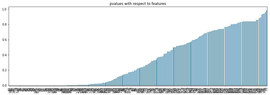
The plot shows a clear gap: a small cluster of features have p-values near zero (very strong signal), while the majority have p-values above 0.5 (noise). The threshold at 0.05 cuts cleanly between the two groups.
Select only the features that have a statistically significant p-value of less than 0.05:
p_values = p_values[p_values<0.05]Print the index of the selected features:
p_values.indexInt64Index([ 40, 182, 86, 22, 101, 51, 2, 127, 49, 91, 30, 27, 61,
52, 23, 85, 56, 25, 54, 29, 58, 28, 57, 185, 119, 111,
26, 55, 16, 17, 13, 21, 14, 69, 33, 184, 32, 68, 223,
178, 109, 224, 36, 34, 15, 18, 44, 168, 221, 198, 199, 100,
196, 197, 244, 46, 24, 53, 62, 31, 125, 38, 144, 50, 108,
220, 115, 219, 183, 35, 98, 172, 60, 59, 217, 180, 95, 92,
166, 72, 105, 209, 202, 211, 186, 212, 70, 110],
dtype='int64')Transform training and testing datasets to retain only the statistically significant features:
X_train_p = X_train_unique[p_values.index]
X_test_p = X_test_unique[p_values.index]
ANOVA reduced the feature set from 227 to 88 — a further 61% reduction while keeping only the features the test deems informative.
Build the Classifiers and Compare Performance
Training a Random Forest — an ensemble of decision trees — on both the full and the reduced feature sets lets you measure the real cost (or benefit) of the selection step. You can learn more about how Random Forests work in Random Forest Classifier and Regressor.
Define the helper function to fit and evaluate the model:
def run_randomForest(X_train, X_test, y_train, y_test):
    clf = RandomForestClassifier(n_estimators=100, random_state=0, n_jobs = -1)
    clf.fit(X_train, y_train)
    y_pred = clf.predict(X_test)
    print('Accuracy: ', accuracy_score(y_test, y_pred))
Train and evaluate the model on the statistically selected feature subset:
%%time
run_randomForest(X_train_p, X_test_p, y_train, y_test)Accuracy: 0.953
Wall time: 814 msTrain and evaluate the model on the full original dataset:
%%time
run_randomForest(X_train, X_test, y_train, y_test)Accuracy: 0.9585
Wall time: 1.49 sThe ANOVA-selected model trains in 814 ms vs. 1.49 s for the full model — nearly twice as fast — while losing only 0.55 percentage points of accuracy (95.3% vs. 95.85%). In production, this trade-off is almost always worthwhile.
Conclusion
In this tutorial you applied univariate ANOVA feature selection to a 370-feature bank dataset. After removing constant, quasi-constant, and duplicate features, f_classif ranked the remaining 227 features by how well their means separated the two target classes. Keeping only those with produced an 88-feature subset. A Random Forest trained on that subset ran nearly twice as fast as one trained on the full set, with an accuracy drop of less than 0.6%.
Key takeaways:
- The ANOVA F-test measures whether a feature's mean differs significantly across target classes, making it a strong filter for classification with continuous features.
- Filter-based methods like ANOVA run independently of any model — they are fast, cheap, and easy to interpret.
- Using as the significance threshold provides a statistically principled cut-off that generalises well across datasets.
- Removing constant and duplicate features before running ANOVA is important — those columns inflate the feature count without providing any discriminatory information.
Next steps:
- Explore Feature Selection Using Mutual Information to capture non-linear relationships between features and the target that ANOVA misses.
- Learn about the ROC-AUC univariate filter in Feature Selection Based on Univariate ROC-AUC for a model-performance-based alternative to statistical testing.
- Apply Lasso regularisation for an embedded selection approach in Lasso and Ridge Regularisation for Feature Selection.

