
When working on a data science project, you spend most of your time cleaning and preprocessing data. Choosing the right library to manipulate tabular data efficiently is crucial for a smooth workflow.
Pandas is the standard open-source library for data analysis and manipulation in Python. Built on top of NumPy, it introduces the DataFrame—a highly optimized two-dimensional tabular data structure with labeled axes (rows and columns) that makes data manipulation fast and intuitive.
In this tutorial, you will build a complete data cleaning and analysis pipeline. You will learn to construct DataFrames from scratch, import real-world datasets like NBA player stats and IMDB movie rankings, handle duplicate rows, impute missing values using statistical means, and analyze variable relationships with correlation.
Prerequisites: Python 3.x, Pandas, NumPy, Seaborn, Matplotlib.
Datasets
You can download all the datasets used in this tutorial from the All CSV ML Data Files Download repository.
Getting Started
To begin working with the library, you must first import the module under its standard alias:
import pandas as pdPrepare a Python dictionary containing lists of values to represent orange and apple counts:
data = {
    'apple': [3,1,4,5],
    'orange': [1, 5, 6, 8]
}

data{'apple': [3, 1, 4, 5], 'orange': [1, 5, 6, 8]}Check the data type of your newly created dictionary:
type(data)dictConvert your Python dictionary into a Pandas DataFrame. A DataFrame is a two-dimensional, size-mutable, and potentially heterogeneous tabular data structure. It aligns data in a tabular fashion using rows and columns:
df = pd.DataFrame(data)
df| apple | orange | |
|---|---|---|
| 0 | 3 | 1 |
| 1 | 1 | 5 |
| 2 | 4 | 6 |
| 3 | 5 | 8 |
Extract a single column to see how Pandas represents individual columns as Series. A Series is a one-dimensional array-like object that contains a sequence of values:
df['apple']0 3
1 1
2 4
3 5
Name: apple, dtype: int64Verify that the type of the extracted column is indeed a Pandas Series:
type(df['apple'])pandas.core.series.SeriesReading CSV Files
To load external datasets, Pandas provides robust input/output functions. For example, read_csv() imports a comma-separated values file directly into a DataFrame:
df = pd.read_csv('nba.csv')Display the first ten rows of the DataFrame using head() to examine the dataset structure:
df.head(10)| Name | Team | Number | Position | Age | Height | Weight | College | Salary | |
|---|---|---|---|---|---|---|---|---|---|
| 0 | Avery Bradley | Boston Celtics | 0.0 | PG | 25.0 | 6-2 | 180.0 | Texas | 7730337.0 |
| 1 | Jae Crowder | Boston Celtics | 99.0 | SF | 25.0 | 6-6 | 235.0 | Marquette | 6796117.0 |
| 2 | John Holland | Boston Celtics | 30.0 | SG | 27.0 | 6-5 | 205.0 | Boston University | NaN |
| 3 | R.J. Hunter | Boston Celtics | 28.0 | SG | 22.0 | 6-5 | 185.0 | Georgia State | 1148640.0 |
| 4 | Jonas Jerebko | Boston Celtics | 8.0 | PF | 29.0 | 6-10 | 231.0 | NaN | 5000000.0 |
| 5 | Amir Johnson | Boston Celtics | 90.0 | PF | 29.0 | 6-9 | 240.0 | NaN | 12000000.0 |
| 6 | Jordan Mickey | Boston Celtics | 55.0 | PF | 21.0 | 6-8 | 235.0 | LSU | 1170960.0 |
| 7 | Kelly Olynyk | Boston Celtics | 41.0 | C | 25.0 | 7-0 | 238.0 | Gonzaga | 2165160.0 |
| 8 | Terry Rozier | Boston Celtics | 12.0 | PG | 22.0 | 6-2 | 190.0 | Louisville | 1824360.0 |
| 9 | Marcus Smart | Boston Celtics | 36.0 | PG | 22.0 | 6-4 | 220.0 | Oklahoma State | 3431040.0 |
View the last two rows of the dataset using tail() to verify row alignments at the end of the file:
df.tail(2)| Name | Team | Number | Position | Age | Height | Weight | College | Salary | |
|---|---|---|---|---|---|---|---|---|---|
| 456 | Jeff Withey | Utah Jazz | 24.0 | C | 26.0 | 7-0 | 231.0 | Kansas | 947276.0 |
| 457 | NaN | NaN | NaN | NaN | NaN | NaN | NaN | NaN | NaN |
Load the CSV file while specifying the Name column to act as the row labels or index of the DataFrame:
df = pd.read_csv('nba.csv', index_col = 'Name')
df.head()| Name | Team | Number | Position | Age | Height | Weight | College | Salary |
|---|---|---|---|---|---|---|---|---|
| Avery Bradley | Boston Celtics | 0.0 | PG | 25.0 | 6-2 | 180.0 | Texas | 7730337.0 |
| Jae Crowder | Boston Celtics | 99.0 | SF | 25.0 | 6-6 | 235.0 | Marquette | 6796117.0 |
| John Holland | Boston Celtics | 30.0 | SG | 27.0 | 6-5 | 205.0 | Boston University | NaN |
| R.J. Hunter | Boston Celtics | 28.0 | SG | 22.0 | 6-5 | 185.0 | Georgia State | 1148640.0 |
| Jonas Jerebko | Boston Celtics | 8.0 | PF | 29.0 | 6-10 | 231.0 | NaN | 5000000.0 |
You can also use custom row labels for other datasets. For example, load the IMDB Movie dataset using the movie's rank as the index:
df = pd.read_csv('IMDB-Movie-Data.csv', index_col = 'Rank')
df.head()| Rank | Title | Genre | Description | Director | Actors | Year | Runtime (Minutes) | Rating | Votes | Revenue (Millions) | Metascore |
|---|---|---|---|---|---|---|---|---|---|---|---|
| 1 | Guardians of the Galaxy | Action,Adventure,Sci-Fi | A group of intergalactic criminals are forced ... | James Gunn | Chris Pratt, Vin Diesel, Bradley Cooper, Zoe S... | 2014 | 121 | 8.1 | 757074 | 333.13 | 76.0 |
| 2 | Prometheus | Adventure,Mystery,Sci-Fi | Following clues to the origin of mankind, a te... | Ridley Scott | Noomi Rapace, Logan Marshall-Green, Michael Fa... | 2012 | 124 | 7.0 | 485820 | 126.46 | 65.0 |
| 3 | Split | Horror,Thriller | Three girls are kidnapped by a man with a diag... | M. Night Shyamalan | James McAvoy, Anya Taylor-Joy, Haley Lu Richar... | 2016 | 117 | 7.3 | 157606 | 138.12 | 62.0 |
| 4 | Sing | Animation,Comedy,Family | In a city of humanoid animals, a hustling thea... | Christophe Lourdelet | Matthew McConaughey,Reese Witherspoon, Seth Ma... | 2016 | 108 | 7.2 | 60545 | 270.32 | 59.0 |
| 5 | Suicide Squad | Action,Adventure,Fantasy | A secret government agency recruits some of th... | David Ayer | Will Smith, Jared Leto, Margot Robbie, Viola D... | 2016 | 123 | 6.2 | 393727 | 325.02 | 40.0 |
Display the last five rows of the IMDB dataset to verify the tail structure:
df.tail()| Rank | Title | Genre | Description | Director | Actors | Year | Runtime (Minutes) | Rating | Votes | Revenue (Millions) | Metascore |
|---|---|---|---|---|---|---|---|---|---|---|---|
| 996 | Secret in Their Eyes | Crime,Drama,Mystery | A tight-knit team of rising investigators, alo... | Billy Ray | Chiwetel Ejiofor, Nicole Kidman, Julia Roberts... | 2015 | 111 | 6.2 | 27585 | NaN | 45.0 |
| 997 | Hostel: Part II | Horror | Three American college students studying abroa... | Eli Roth | Lauren German, Heather Matarazzo, Bijou Philli... | 2007 | 94 | 5.5 | 73152 | 17.54 | 46.0 |
| 998 | Step Up 2: The Streets | Drama,Music,Romance | Romantic sparks occur between two dance studen... | Jon M. Chu | Robert Hoffman, Briana Evigan, Cassie Ventura,... | 2008 | 98 | 6.2 | 70699 | 58.01 | 50.0 |
| 999 | Search Party | Adventure,Comedy | A pair of friends embark on a mission to reuni... | Scot Armstrong | Adam Pally, T.J. Miller, Thomas Middleditch,Sh... | 2014 | 93 | 5.6 | 4881 | NaN | 22.0 |
| 1000 | Nine Lives | Comedy,Family,Fantasy | A stuffy businessman finds himself trapped ins... | Barry Sonnenfeld | Kevin Spacey, Jennifer Garner, Robbie Amell,Ch... | 2016 | 87 | 5.3 | 12435 | 19.64 | 11.0 |
To inspect the schema, data types, and non-null counts of each column, call the info() method:
df.info()Int64Index: 1000 entries, 1 to 1000
Data columns (total 11 columns):
Title 1000 non-null object
Genre 1000 non-null object
Description 1000 non-null object
Director 1000 non-null object
Actors 1000 non-null object
Year 1000 non-null int64
Runtime (Minutes) 1000 non-null int64
Rating 1000 non-null float64
Votes 1000 non-null int64
Revenue (Millions) 872 non-null float64
Metascore 936 non-null float64
dtypes: float64(3), int64(3), object(5)
memory usage: 93.8+ KBTo check the dimensionality of the DataFrame, inspect the shape attribute:
df.shape(1000, 11)You can count duplicate rows by combining the duplicated() method with a sum operation:
sum(df.duplicated())0To demonstrate duplicate handling, append the DataFrame to itself to double the number of rows:
df1 = df.append(df)
df1.shape(2000, 11)Verify the number of duplicate rows in the newly concatenated DataFrame:
df1.duplicated().sum()1000Remove the duplicate rows using drop_duplicates() to return a cleaned copy:
df2 = df1.drop_duplicates()
df2.shape(1000, 11)Note that the original DataFrame remains unchanged unless you assign the result back or modify it in place:
df1.shape(2000, 11)To modify the DataFrame directly without creating a new copy, set the inplace parameter to True:
df1.drop_duplicates(inplace = True)
df1.shape(1000, 11)Column Operations
Access the column labels of the DataFrame using the columns attribute:
df.columnsIndex(['Title', 'Genre', 'Description', 'Director', 'Actors', 'Year',
'Runtime (Minutes)', 'Rating', 'Votes', 'Revenue (Millions)',
'Metascore'],
dtype='object')Count the number of columns in the DataFrame:
len(df.columns)11Generate descriptive statistics for the numerical columns using the describe() method:
df.describe()| Year | Runtime (Minutes) | Rating | Votes | Revenue (Millions) | Metascore | |
|---|---|---|---|---|---|---|
| count | 1000.000000 | 1000.000000 | 1000.000000 | 1.000000e+03 | 872.000000 | 936.000000 |
| mean | 2012.783000 | 113.172000 | 6.723200 | 1.698083e+05 | 82.956376 | 58.985043 |
| std | 3.205962 | 18.810908 | 0.945429 | 1.887626e+05 | 103.253540 | 17.194757 |
| min | 2006.000000 | 66.000000 | 1.900000 | 6.100000e+01 | 0.000000 | 11.000000 |
| 25% | 2010.000000 | 100.000000 | 6.200000 | 3.630900e+04 | 13.270000 | 47.000000 |
| 50% | 2014.000000 | 111.000000 | 6.800000 | 1.107990e+05 | 47.985000 | 59.500000 |
| 75% | 2016.000000 | 123.000000 | 7.400000 | 2.399098e+05 | 113.715000 | 72.000000 |
| max | 2016.000000 | 191.000000 | 9.000000 | 1.791916e+06 | 936.630000 | 100.000000 |
Extract the column names and convert them into a standard Python list:
col = df.columns
type(list(col))listDisplay the index object containing all column names:
colIndex(['Title', 'Genre', 'Description', 'Director', 'Actors', 'Year',
'Runtime (Minutes)', 'Rating', 'Votes', 'Revenue (Millions)',
'Metascore'],
dtype='object')You can rename columns by assigning a list of new names directly to the columns attribute:
col1 = ['a', 'b', 'c', 'd', 'e', 'f', 'g', 'h', 'i', 'j', 'k']
df.columns = col1
df.head()| Rank | a | b | c | d | e | f | g | h | i | j | k |
|---|---|---|---|---|---|---|---|---|---|---|---|
| 1 | Guardians of the Galaxy | Action,Adventure,Sci-Fi | A group of intergalactic criminals are forced ... | James Gunn | Chris Pratt, Vin Diesel, Bradley Cooper, Zoe S... | 2014 | 121 | 8.1 | 757074 | 333.13 | 76.0 |
| 2 | Prometheus | Adventure,Mystery,Sci-Fi | Following clues to the origin of mankind, a te... | Ridley Scott | Noomi Rapace, Logan Marshall-Green, Michael Fa... | 2012 | 124 | 7.0 | 485820 | 126.46 | 65.0 |
| 3 | Split | Horror,Thriller | Three girls are kidnapped by a man with a diag... | M. Night Shyamalan | James McAvoy, Anya Taylor-Joy, Haley Lu Richar... | 2016 | 117 | 7.3 | 157606 | 138.12 | 62.0 |
| 4 | Sing | Animation,Comedy,Family | In a city of humanoid animals, a hustling thea... | Christophe Lourdelet | Matthew McConaughey,Reese Witherspoon, Seth Ma... | 2016 | 108 | 7.2 | 60545 | 270.32 | 59.0 |
| 5 | Suicide Squad | Action,Adventure,Fantasy | A secret government agency recruits some of th... | David Ayer | Will Smith, Jared Leto, Margot Robbie, Viola D... | 2016 | 123 | 6.2 | 393727 | 325.02 | 40.0 |
Revert back to the original column names:
df.columns = col
df.head(0)| Rank | Title | Genre | Description | Director | Actors | Year | Runtime (Minutes) | Rating | Votes | Revenue (Millions) | Metascore |
|---|
For more precise renaming, use the rename() method with a dictionary mapping old column names to new ones:
df.rename(columns={
    'Runtime (Minutes)': 'Runtime',
    'Revenue (Millions)': 'Revenue'
}, inplace= True)

df.columnsIndex(['Title', 'Genre', 'Description', 'Director', 'Actors', 'Year',
'Runtime', 'Rating', 'Votes', 'Revenue', 'Metascore'],
dtype='object')Compare the updated column list with the original stored in the col variable:
colIndex(['Title', 'Genre', 'Description', 'Director', 'Actors', 'Year',
'Runtime (Minutes)', 'Rating', 'Votes', 'Revenue (Millions)',
'Metascore'],
dtype='object')Missing Values
Real-world datasets often contain missing values. You can represent these missing entries in Python using NumPy's nan constant:
import numpy as npAccess the standard representation for empty values:
np.nannanIdentify missing values in the DataFrame using isnull(), which returns boolean values indicating the presence of null values:
df.isnull().head(10)| Rank | Title | Genre | Description | Director | Actors | Year | Runtime | Rating | Votes | Revenue | Metascore |
|---|---|---|---|---|---|---|---|---|---|---|---|
| 1 | False | False | False | False | False | False | False | False | False | False | False |
| 2 | False | False | False | False | False | False | False | False | False | False | False |
| 3 | False | False | False | False | False | False | False | False | False | False | False |
| 4 | False | False | False | False | False | False | False | False | False | False | False |
| 5 | False | False | False | False | False | False | False | False | False | False | False |
| 6 | False | False | False | False | False | False | False | False | False | False | False |
| 7 | False | False | False | False | False | False | False | False | False | False | False |
| 8 | False | False | False | False | False | False | False | False | False | True | False |
| 9 | False | False | False | False | False | False | False | False | False | False | False |
| 10 | False | False | False | False | False | False | False | False | False | False | False |
Sum the boolean values to count the number of missing records in each column:
df.isnull().sum()Title 0
Genre 0
Description 0
Director 0
Actors 0
Year 0
Runtime 0
Rating 0
Votes 0
Revenue 128
Metascore 64
dtype: int64Alternatively, call isna() to achieve the same result:
df.isna().sum()Title 0
Genre 0
Description 0
Director 0
Actors 0
Year 0
Runtime 0
Rating 0
Votes 0
Revenue 128
Metascore 64
dtype: int64Remove any rows containing at least one missing value using dropna():
df1 = df.dropna()
df1.shape(838, 11)To drop columns that contain missing values instead of rows, set axis=1:
df2 = df.dropna(axis = 1)
df2.head(3)| Rank | Title | Genre | Description | Director | Actors | Year | Runtime | Rating | Votes |
|---|---|---|---|---|---|---|---|---|---|
| 1 | Guardians of the Galaxy | Action,Adventure,Sci-Fi | A group of intergalactic criminals are forced ... | James Gunn | Chris Pratt, Vin Diesel, Bradley Cooper, Zoe S... | 2014 | 121 | 8.1 | 757074 |
| 2 | Prometheus | Adventure,Mystery,Sci-Fi | Following clues to the origin of mankind, a te... | Ridley Scott | Noomi Rapace, Logan Marshall-Green, Michael Fa... | 2012 | 124 | 7.0 | 485820 |
| 3 | Split | Horror,Thriller | Three girls are kidnapped by a man with a diag... | M. Night Shyamalan | James McAvoy, Anya Taylor-Joy, Haley Lu Richar... | 2016 | 117 | 7.3 | 157606 |
Imputation
Rather than deleting rows or columns, you can fill missing cells with a specific value. Fill all missing entries with 0 using fillna():
df3 = df.fillna(0)
df3.isna().sum()Title 0
Genre 0
Description 0
Director 0
Actors 0
Year 0
Runtime 0
Rating 0
Votes 0
Revenue 0
Metascore 0
dtype: int64Recall the counts of null values in the original DataFrame:
df.isnull().sum()Title 0
Genre 0
Description 0
Director 0
Actors 0
Year 0
Runtime 0
Rating 0
Votes 0
Revenue 128
Metascore 64
dtype: int64Extract the Revenue column as a Pandas Series:
revenue = df['Revenue']
type(revenue)pandas.core.series.SeriesDisplay the last five elements of the revenue Series to check for missing entries:
revenue.tail()Rank
996 NaN
997 17.54
998 58.01
999 NaN
1000 19.64
Name: Revenue, dtype: float64Compute the average revenue to use for imputation:
revenue_mean = revenue.mean()
revenue_mean82.95637614678897Fill the missing entries in revenue with its calculated mean value in-place:
revenue.fillna(revenue_mean, inplace= True)
revenue.tail()Rank
996 82.956376
997 17.540000
998 58.010000
999 82.956376
1000 19.640000
Name: Revenue, dtype: float64Confirm that the revenue Series no longer contains null values:
revenue.isnull().sum()0Assign the imputed Series back to the DataFrame and check the remaining null counts:
df['Revenue'] = revenue
df.isnull().sum()Title 0
Genre 0
Description 0
Director 0
Actors 0
Year 0
Runtime 0
Rating 0
Votes 0
Revenue 0
Metascore 64
dtype: int64Apply the same mean-imputation process to the Metascore column:
metascore = df['Metascore']
metascore_mean = metascore.mean()
print("metascore_mean =",metascore_mean)
metascore.fillna(metascore_mean, inplace = True)
df['Metascore'] = metascore
df.isnull().sum()metascore_mean = 58.98504273504273
Title          0
Genre          0
Description    0
Director       0
Actors         0
Year           0
Runtime        0
Rating         0
Votes          0
Revenue        0
Metascore      0
dtype: int64Verify the statistical summary of the numerical columns now that the missing values are imputed:
df.describe()| Year | Runtime | Rating | Votes | Revenue | Metascore | |
|---|---|---|---|---|---|---|
| count | 1000.000000 | 1000.000000 | 1000.000000 | 1.000000e+03 | 1000.000000 | 1000.000000 |
| mean | 2012.783000 | 113.172000 | 6.723200 | 1.698083e+05 | 82.956376 | 58.985043 |
| std | 3.205962 | 18.810908 | 0.945429 | 1.887626e+05 | 96.412043 | 16.634858 |
| min | 2006.000000 | 66.000000 | 1.900000 | 6.100000e+01 | 0.000000 | 11.000000 |
| 25% | 2010.000000 | 100.000000 | 6.200000 | 3.630900e+04 | 17.442500 | 47.750000 |
| 50% | 2014.000000 | 111.000000 | 6.800000 | 1.107990e+05 | 60.375000 | 58.985043 |
| 75% | 2016.000000 | 123.000000 | 7.400000 | 2.399098e+05 | 99.177500 | 71.000000 |
| max | 2016.000000 | 191.000000 | 9.000000 | 1.791916e+06 | 936.630000 | 100.000000 |
Print the updated info schema to confirm all columns have 1000 non-null values:
df.info()Int64Index: 1000 entries, 1 to 1000
Data columns (total 11 columns):
Title 1000 non-null object
Genre 1000 non-null object
Description 1000 non-null object
Director 1000 non-null object
Actors 1000 non-null object
Year 1000 non-null int64
Runtime 1000 non-null int64
Rating 1000 non-null float64
Votes 1000 non-null int64
Revenue 1000 non-null float64
Metascore 1000 non-null float64
dtypes: float64(3), int64(3), object(5)
memory usage: 93.8+ KBGet a statistical summary of the non-numerical Genre column:
df['Genre'].describe()count 1000
unique 207
top Action,Adventure,Sci-Fi
freq 50
Name: Genre, dtype: objectCount the frequencies of the top ten movie genres:
df['Genre'].value_counts().head(10)Action,Adventure,Sci-Fi 50
Drama 48
Comedy,Drama,Romance 35
Comedy 32
Drama,Romance 31
Comedy,Drama 27
Action,Adventure,Fantasy 27
Animation,Adventure,Comedy 27
Comedy,Romance 26
Crime,Drama,Thriller 24
Name: Genre, dtype: int64Check the count of unique movie genres present in the dataset:
len(df['Genre'].unique())207Correlation Analysis
Compute the pairwise Pearson correlation matrix for the numerical columns using the corr() method:
corrmat = df.corr()
corrmat| Year | Runtime | Rating | Votes | Revenue | Metascore | |
|---|---|---|---|---|---|---|
| Year | 1.000000 | -0.164900 | -0.211219 | -0.411904 | -0.117562 | -0.076077 |
| Runtime | -0.164900 | 1.000000 | 0.392214 | 0.407062 | 0.247834 | 0.202239 |
| Rating | -0.211219 | 0.392214 | 1.000000 | 0.511537 | 0.189527 | 0.604723 |
| Votes | -0.411904 | 0.407062 | 0.511537 | 1.000000 | 0.607941 | 0.318116 |
| Revenue | -0.117562 | 0.247834 | 0.189527 | 0.607941 | 1.000000 | 0.132304 |
| Metascore | -0.076077 | 0.202239 | 0.604723 | 0.318116 | 0.132304 | 1.000000 |
You can compute relationships between numerical attributes using correlation matrices. To visualize these correlation matrices as colors, import the Seaborn library:
import seaborn as snsPlot the correlation matrix as a color-encoded heat map:
sns.heatmap(corrmat)You can also use Matplotlib to generate visualizations directly from DataFrames. Import the Matplotlib pyplot interface:
import matplotlib.pyplot as pltGenerate a scatter plot of movie ratings versus revenues:
df.plot(kind = 'scatter', x = 'Rating', y = 'Revenue', title = 'Revenue vs Rating')Create a histogram plot to view the frequency distribution of ratings:
df['Rating'].plot(kind = 'hist', title = 'Rating')Estimate the probability density of ratings using a Kernel Density Estimation (KDE) plot:
df['Rating'].plot(kind = 'kde', title = 'Rating')Count the frequency of each rating category:
df['Rating'].value_counts()7.1 52
6.7 48
7.0 46
6.3 44
6.6 42
7.2 42
7.3 42
6.5 40
7.8 40
6.2 37
6.8 37
7.5 35
6.4 35
7.4 33
6.9 31
6.1 31
7.6 27
7.7 27
5.8 26
6.0 26
8.1 26
7.9 23
5.7 21
8.0 19
5.9 19
5.6 17
5.5 14
5.3 12
5.4 12
5.2 11
8.2 10
4.9 7
8.3 7
4.7 6
8.5 6
4.6 5
5.1 5
5.0 4
4.8 4
4.3 4
8.4 4
3.9 3
8.6 3
8.8 2
2.7 2
4.2 2
3.5 2
3.7 2
9.0 1
3.2 1
4.0 1
4.5 1
4.4 1
4.1 1
1.9 1
Name: Rating, dtype: int64To visualize the distribution, spread, and outliers of ratings, you can construct a box plot. Box plots represent the five-number summary of a dataset: the minimum, first quartile (), median, third quartile (), and maximum:
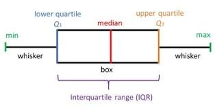
Generate a box plot of movie ratings:
df['Rating'].plot(kind = 'box')Compute numerical statistics for movie ratings to match the box plot coordinates:
df['Rating'].describe()count 1000.000000
mean 6.723200
std 0.945429
min 1.900000
25% 6.200000
50% 6.800000
75% 7.400000
max 9.000000
Name: Rating, dtype: float64Add a new rating category column to label movies as good or bad depending on their rating threshold:
rating_cat = []
for rate in df['Rating']:
    if rate > 6.2:
        rating_cat.append('Good')
    else:
        rating_cat.append('Bad')

rating_cat[:20]['Good', 'Good', 'Good', 'Good', 'Bad', 'Bad', 'Good', 'Good', 'Good', 'Good', 'Good', 'Good', 'Good', 'Good', 'Good', 'Good', 'Good', 'Good', 'Good', 'Good']Assign the list to the DataFrame and display the head to confirm the column addition:
df['Rating Category'] = rating_cat
df.head()| Rank | Title | Genre | Description | Director | Actors | Year | Runtime | Rating | Votes | Revenue | Metascore | Rating Category |
|---|---|---|---|---|---|---|---|---|---|---|---|---|
| 1 | Guardians of the Galaxy | Action,Adventure,Sci-Fi | A group of intergalactic criminals are forced ... | James Gunn | Chris Pratt, Vin Diesel, Bradley Cooper, Zoe S... | 2014 | 121 | 8.1 | 757074 | 333.13 | 76.0 | Good |
| 2 | Prometheus | Adventure,Mystery,Sci-Fi | Following clues to the origin of mankind, a te... | Ridley Scott | Noomi Rapace, Logan Marshall-Green, Michael Fa... | 2012 | 124 | 7.0 | 485820 | 126.46 | 65.0 | Good |
| 3 | Split | Horror,Thriller | Three girls are kidnapped by a man with a diag... | M. Night Shyamalan | James McAvoy, Anya Taylor-Joy, Haley Lu Richar... | 2016 | 117 | 7.3 | 157606 | 138.12 | 62.0 | Good |
| 4 | Sing | Animation,Comedy,Family | In a city of humanoid animals, a hustling thea... | Christophe Lourdelet | Matthew McConaughey,Reese Witherspoon, Seth Ma... | 2016 | 108 | 7.2 | 60545 | 270.32 | 59.0 | Good |
| 5 | Suicide Squad | Action,Adventure,Fantasy | A secret government agency recruits some of th... | David Ayer | Will Smith, Jared Leto, Margot Robbie, Viola D... | 2016 | 123 | 6.2 | 393727 | 325.02 | 40.0 | Bad |
Group your data by a categorical feature and draw box plots for each group using the boxplot() method:
df.boxplot(column= 'Revenue', by = 'Rating Category')Conclusion
In this tutorial, you explored the core functionalities of the Pandas library, including DataFrame creation, duplicate removal, column renaming, and handling missing values using mean imputation. Using the NBA and IMDB datasets, you walked through essential data cleaning steps and calculated pairwise correlation to assess linear dependencies between numeric variables.
Key takeaways:
- DataFrames and Series: A DataFrame is a two-dimensional tabular structure, while a Series represents a single column within that DataFrame.
- Wrangling and Deduplication: Tabular data often contains duplicates that can be filtered out using
drop_duplicates(inplace=True)to clean the workspace. - Handling Null Values: Missing data (
NaN) should either be dropped or imputed using operations likefillna()with statistical metrics such as the column mean. - Correlation: The
corr()method helps calculate pairwise relationship coefficients to find dependencies before building predictive models.
Next steps:
- Dive deeper into visual analysis with Data Visualization with Pandas to learn how to plot line, bar, scatter, and area graphs directly from DataFrames.
- Master plotting basics with Matplotlib Crash Course to customize your plots with titles, axes, and styles.
- Learn about the different kinds of variables you will encounter in Data Variable Types Every Data Scientist Needs to choose appropriate visualization tools.

