
When you have hundreds of features in a dataset, many of them carry little or no useful information. Training a model on all of them wastes time and can hurt performance. Univariate feature selection is a simple remedy: you score each feature on its own, rank them, and keep only the ones that score well.
This tutorial covers two scoring methods. For binary classification — predicting one of two outcomes — we score each feature by its ROC-AUC (Receiver Operating Characteristic — Area Under the Curve). A score above 0.5 means the feature carries signal; exactly 0.5 means it is no better than a random guess. For regression — predicting a continuous number — we score each feature by its Mean Squared Error (MSE): the lower the error, the stronger the feature's individual relationship with the target.
You will work through two complete examples: a 370-feature bank classification dataset and the 13-feature Boston Housing dataset. By the end you will have reduced both datasets to their most informative features and confirmed that the smaller sets retain nearly all predictive power.
Prerequisites: Python 3.x, Scikit-learn, Pandas, NumPy, Matplotlib, Seaborn.
You can also
.Understanding ROC-AUC
The ROC curve plots the True Positive Rate (the fraction of actual positives that the model correctly identifies) against the False Positive Rate (the fraction of actual negatives that the model incorrectly flags as positive) at every possible classification threshold.
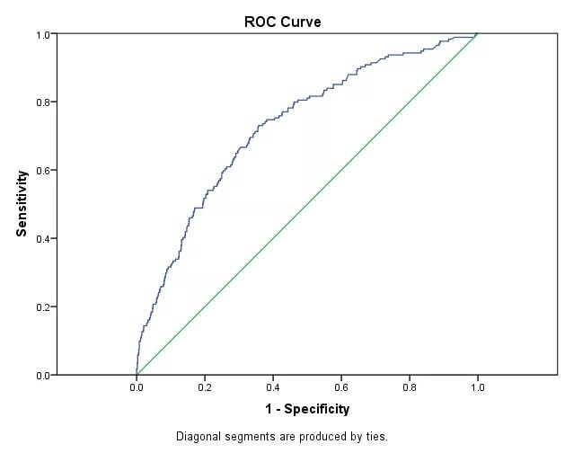
The plot below shows a typical ROC curve. The blue line is the model; the green diagonal is a random classifier with AUC = 0.5. The further the blue line bows toward the top-left corner, the better the model:
The AUC (Area Under the Curve) summarises the entire curve in a single number:
Where:
- — a value between 0 and 1; 1 is a perfect classifier, 0.5 is random, below 0.5 means the model is worse than random
- — True Positive Rate at decision threshold : the fraction of genuine positives correctly predicted
- — False Positive Rate at threshold : the fraction of genuine negatives incorrectly predicted as positive
In this tutorial, we fit a Random Forest on a single feature at a time and record the resulting AUC as that feature's score. Features that score above 0.5 are kept; the rest are discarded.
Use of ROC-AUC in Classification Feature Selection
Import the required libraries for data structures, visualization, and calculation:
import numpy as np
import pandas as pd
import matplotlib.pyplot as plt
import seaborn as sns
Import Scikit-learn packages for validation, metrics, and models:
from sklearn.model_selection import train_test_split
from sklearn.ensemble import RandomForestClassifier
from sklearn.metrics import accuracy_score, roc_auc_score
from sklearn.feature_selection import VarianceThreshold
The dataset used in this section is available at laxmimerit/Data-Files-for-Feature-Selection on GitHub.
Load the classification dataset and inspect its first rows:
data = pd.read_csv('train.csv', nrows = 20000)
data.head()| ID | var3 | var15 | imp_ent_var16_ult1 | imp_op_var39_comer_ult1 | imp_op_var39_comer_ult3 | imp_op_var40_comer_ult1 | imp_op_var40_comer_ult3 | imp_op_var40_efect_ult1 | imp_op_var40_efect_ult3 | ... | saldo_medio_var33_hace2 | saldo_medio_var33_hace3 | saldo_medio_var33_ult1 | saldo_medio_var33_ult3 | saldo_medio_var44_hace2 | saldo_medio_var44_hace3 | saldo_medio_var44_ult1 | saldo_medio_var44_ult3 | var38 | TARGET | |
|---|---|---|---|---|---|---|---|---|---|---|---|---|---|---|---|---|---|---|---|---|---|
| 0 | 1 | 2 | 23 | 0.0 | 0.0 | 0.0 | 0.0 | 0.0 | 0 | 0 | ... | 0.0 | 0.0 | 0.0 | 0.0 | 0.0 | 0.0 | 0.0 | 0.0 | 39205.170000 | 0 |
| 1 | 3 | 2 | 34 | 0.0 | 0.0 | 0.0 | 0.0 | 0.0 | 0 | 0 | ... | 0.0 | 0.0 | 0.0 | 0.0 | 0.0 | 0.0 | 0.0 | 0.0 | 49278.030000 | 0 |
| 2 | 4 | 2 | 23 | 0.0 | 0.0 | 0.0 | 0.0 | 0.0 | 0 | 0 | ... | 0.0 | 0.0 | 0.0 | 0.0 | 0.0 | 0.0 | 0.0 | 0.0 | 67333.770000 | 0 |
| 3 | 8 | 2 | 37 | 0.0 | 195.0 | 195.0 | 0.0 | 0.0 | 0 | 0 | ... | 0.0 | 0.0 | 0.0 | 0.0 | 0.0 | 0.0 | 0.0 | 0.0 | 64007.970000 | 0 |
| 4 | 10 | 2 | 37 | 0.0 | 0.0 | 0.0 | 0.0 | 0.0 | 0 | 0 | ... | 0.0 | 0.0 | 0.0 | 0.0 | 0.0 | 0.0 | 0.0 | 0.0 | 117310.979016 | 0 |
Separate features from the target column and confirm the dataset dimensions:
X = data.drop('TARGET', axis = 1)
y = data['TARGET']
X.shape, y.shape((20000, 370), (20000,))Split the data into 80% training and 20% test sets, stratifying on class labels so that both splits preserve the same class balance:
X_train, X_test, y_train, y_test = train_test_split(X, y, test_size = 0.2, random_state = 0, stratify = y)Remove Constant, Quasi-Constant, and Duplicate Features
Before scoring features by ROC-AUC, remove any features that carry no variance — they cannot possibly be useful predictors. You can also
for a detailed walkthrough of this step.Apply a 1% variance threshold to filter out constant and quasi-constant features. Any feature where more than 99% of values are identical is removed:
#remove constant and quasi constant features
constant_filter = VarianceThreshold(threshold=0.01)
constant_filter.fit(X_train)
X_train_filter = constant_filter.transform(X_train)
X_test_filter = constant_filter.transform(X_test)
X_train_filter.shape, X_test_filter.shape((16000, 245), (4000, 245))Check how many features were removed by the variance filter:
370-245125The variance filter removed 125 features. The remaining 245 still include duplicates — pairs of columns that are byte-for-byte identical and therefore add no new information.
For more details on constant and duplicate removal, see Constant, Quasi-Constant, and Duplicate Feature Removal.
Transpose the filtered datasets so that each feature becomes a row, making it straightforward to identify and drop duplicate rows:
#remove duplicate features
X_train_T = X_train_filter.T
X_test_T = X_test_filter.T
X_train_T = pd.DataFrame(X_train_T)
X_test_T = pd.DataFrame(X_test_T)
Count the number of duplicate feature rows in the training set:
X_train_T.duplicated().sum()18Mark which rows (features) are duplicates:
duplicated_features = X_train_T.duplicated()Keep only the unique features and transpose back to the original shape — rows as samples, columns as features:
features_to_keep = [not index for index in duplicated_features]
X_train_unique = X_train_T[features_to_keep].T
X_test_unique = X_test_T[features_to_keep].T
X_train_unique.shape, X_train.shape((16000, 227), (16000, 370))After removing constant, quasi-constant, and duplicate features, you are left with 227 unique informative features — down from the original 370.
Calculate ROC-AUC Score per Feature
With the reduced feature set ready, score each remaining feature individually. The loop below fits a RandomForestClassifier on a single feature at a time, predicts on the test set, and records the ROC-AUC score:
roc_auc = []
for feature in X_train_unique.columns:
    clf = RandomForestClassifier(n_estimators=100, random_state=0)
    clf.fit(X_train_unique[feature].to_frame(), y_train)
    y_pred = clf.predict(X_test_unique[feature].to_frame())
    roc_auc.append(roc_auc_score(y_test, y_pred))
Print the full list of ROC-AUC scores — one value per feature:
print(roc_auc)[0.5020561820568537, 0.5, 0.5, 0.49986968986187125, 0.501373452866903, 0.49569976544175137, 0.5028068643863192, 0.49986968986187125, 0.5, 0.5, 0.4997393797237425, 0.5017643832812891, 0.49569976544175137, 0.49960906958561374, 0.49895751889497003, 0.49700286682303885, 0.49960906958561374, 0.5021553136956755, 0.4968725566849101, 0.5, 0.5, 0.5, 0.5, 0.5, 0.5, 0.5, 0.5, 0.5, 0.5, 0.5, 0.5, 0.5, 0.5, 0.5, 0.5, 0.5, 0.5, 0.5, 0.5, 0.5, 0.5, 0.5, 0.5, 0.5, 0.5, 0.5, 0.5, 0.5, 0.5, 0.5, 0.5, 0.5, 0.5, 0.5, 0.5, 0.5, 0.5, 0.5, 0.5, 0.5, 0.5, 0.5, 0.5, 0.5, 0.5, 0.5, 0.5, 0.5, 0.5, 0.5, 0.49986968986187125, 0.5, 0.5, 0.5, 0.5, 0.5, 0.5, 0.5, 0.5, 0.5, 0.5, 0.5, 0.5, 0.5, 0.5, 0.5, 0.5, 0.5, 0.5, 0.5, 0.5, 0.5, 0.5, 0.5029371745244479, 0.4959603857180089, 0.5, 0.5048318679438659, 0.4997393797237425, 0.5, 0.5, 0.5, 0.5, 0.5, 0.5, 0.5, 0.49921813917122754, 0.49921813917122754, 0.49824600955181303, 0.5, 0.5, 0.5, 0.4990878290330988, 0.4983763196899418, 0.5, 0.5, 0.5, 0.5, 0.5, 0.5, 0.5, 0.5, 0.5, 0.5, 0.5, 0.5, 0.5, 0.5, 0.5, 0.5, 0.5, 0.5, 0.5, 0.5, 0.5, 0.5, 0.5, 0.5, 0.5025462441100617, 0.4990878290330988, 0.5, 0.5, 0.5, 0.5, 0.5, 0.5, 0.5, 0.5, 0.5, 0.5, 0.5, 0.5, 0.5, 0.5, 0.5, 0.5, 0.5, 0.5, 0.49986968986187125, 0.5, 0.5, 0.5, 0.5, 0.5, 0.5, 0.5, 0.5, 0.5, 0.5, 0.5, 0.5, 0.5, 0.5, 0.5, 0.5, 0.5, 0.5, 0.5, 0.5, 0.5, 0.5, 0.5, 0.5, 0.5, 0.5, 0.5, 0.5, 0.5, 0.4997393797237425, 0.5, 0.5, 0.49986968986187125, 0.4991581805187143, 0.4988272087568413, 0.49674224654678134, 0.4995491109331005, 0.5, 0.5, 0.5022856238338043, 0.5012431427287742, 0.5, 0.5, 0.5, 0.49986968986187125, 0.5, 0.4997393797237425, 0.5, 0.5, 0.5, 0.5, 0.5, 0.5, 0.5, 0.5, 0.5, 0.5, 0.5, 0.5, 0.5, 0.5, 0.5, 0.5, 0.5, 0.5, 0.5, 0.5, 0.5, 0.5076595179963898]Convert the list to a Pandas Series, align it with the feature column names, and sort from highest to lowest score:
roc_values = pd.Series(roc_auc)
roc_values.index = X_train_unique.columns
roc_values.sort_values(ascending =False, inplace = True)
Inspect the sorted ROC-AUC values:
roc_values244 0.507660
107 0.504832
104 0.502937
6 0.502807
155 0.502546
...
18 0.496873
211 0.496742
105 0.495960
12 0.495700
5 0.495700
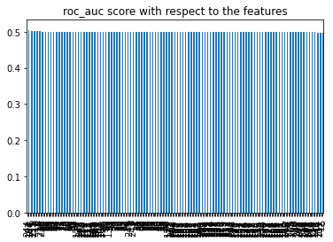
Length: 227, dtype: float64Features with a score of 0.5 or below offer no predictive value above random chance. The bar plot below confirms that the vast majority of features cluster right at 0.5, with only a handful rising above it:
Filter the Series to keep only features that score above 0.5:
sel = roc_values[roc_values>0.5]
sel244 0.507660
107 0.504832
104 0.502937
6 0.502807
155 0.502546
215 0.502286
17 0.502155
0 0.502056
11 0.501764
4 0.501373
216 0.501243
dtype: float64Eleven features survive the ROC-AUC filter. Build the reduced training and test sets using those feature indices:
X_train_roc = X_train_unique[sel.index]
X_test_roc = X_test_unique[sel.index]
Compare Model Performance Before and After Selection
To confirm the selection is meaningful, train a RandomForestClassifier on both the reduced set and the original full set and compare accuracy and training time.
Define a reusable helper function that fits the classifier and prints accuracy:
def run_randomForest(X_train, X_test, y_train, y_test):
    clf = RandomForestClassifier(n_estimators=100, random_state=0, n_jobs=-1)
    clf.fit(X_train, y_train)
    y_pred = clf.predict(X_test)
    print('Accuracy on test set: ', accuracy_score(y_test, y_pred))
Train and evaluate using only the 11 ROC-AUC-selected features:
%%time
run_randomForest(X_train_roc, X_test_roc, y_train, y_test)Accuracy on test set: 0.95275
Wall time: 917 msCheck the shape of the selected feature space to confirm you are working with 11 features:
X_train_roc.shape(16000, 11)Train and evaluate using the full original 370 features as a baseline:
%%time
run_randomForest(X_train, X_test, y_train, y_test)Accuracy on test set: 0.9585
Wall time: 1.76 sUsing only 11 features instead of 370 cuts training time from 1.76 s to 917 ms while losing only 0.58 percentage points of accuracy — a strong trade-off for most real-world pipelines.
Feature Selection Using MSE in Regression
Univariate performance-based selection works for regression too. Instead of AUC, we measure Mean Squared Error (MSE) — the average squared difference between predicted and actual values. A feature with low MSE has a strong individual linear relationship with the target; a high MSE means the feature is a weak predictor on its own.
The MSE formula is:
Where:
- — the number of samples in the test set
- — the actual target value for sample
- — the predicted target value for sample
- — the average squared prediction error; lower values indicate a better-fitting feature
Import the packages for linear modeling and regression metrics:
from sklearn.datasets import load_boston
from sklearn.linear_model import LinearRegressionfrom sklearn.metrics import mean_absolute_error, mean_squared_error, r2_scoreLoad the Boston Housing dataset and print its description to understand the 13 available features:
boston = load_boston()
print(boston.DESCR).. _boston_dataset:
Boston house prices dataset
---------------------------
**Data Set Characteristics:**
:Number of Instances: 506
:Number of Attributes: 13 numeric/categorical predictive. Median Value (attribute 14) is usually the target.
:Attribute Information (in order):
- CRIM per capita crime rate by town
- ZN proportion of residential land zoned for lots over 25,000 sq.ft.
- INDUS proportion of non-retail business acres per town
- CHAS Charles River dummy variable (= 1 if tract bounds river; 0 otherwise)
- NOX nitric oxides concentration (parts per 10 million)
- RM average number of rooms per dwelling
- AGE proportion of owner-occupied units built prior to 1940
- DIS weighted distances to five Boston employment centres
- RAD index of accessibility to radial highways
- TAX full-value property-tax rate per $10,000
- PTRATIO pupil-teacher ratio by town
- B 1000(Bk - 0.63)^2 where Bk is the proportion of blacks by town
- LSTAT % lower status of the population
- MEDV Median value of owner-occupied homes in $1000's
:Missing Attribute Values: None
:Creator: Harrison, D. and Rubinfeld, D.L.
This is a copy of UCI ML housing dataset.
https://archive.ics.uci.edu/ml/machine-learning-databases/housing/
This dataset was taken from the StatLib library which is maintained at Carnegie Mellon University.
The Boston house-price data of Harrison, D. and Rubinfeld, D.L. 'Hedonic
prices and the demand for clean air', J. Environ. Economics & Management,
vol.5, 81-102, 1978. Used in Belsley, Kuh & Welsch, 'Regression diagnostics
...', Wiley, 1980. N.B. Various transformations are used in the table on
pages 244-261 of the latter.
The Boston house-price data has been used in many machine learning papers that address regression
problems.
.. topic:: References
- Belsley, Kuh & Welsch, 'Regression diagnostics: Identifying Influential Data and Sources of Collinearity', Wiley, 1980. 244-261.
- Quinlan,R. (1993). Combining Instance-Based and Model-Based Learning. In Proceedings on the Tenth International Conference of Machine Learning, 236-243, University of Massachusetts, Amherst. Morgan Kaufmann.Create a Pandas DataFrame from the feature matrix and inspect the first rows:
X = pd.DataFrame(boston.data, columns=boston.feature_names)
X.head()| CRIM | ZN | INDUS | CHAS | NOX | RM | AGE | DIS | RAD | TAX | PTRATIO | B | LSTAT | |
|---|---|---|---|---|---|---|---|---|---|---|---|---|---|
| 0 | 0.00632 | 18.0 | 2.31 | 0.0 | 0.538 | 6.575 | 65.2 | 4.0900 | 1.0 | 296.0 | 15.3 | 396.90 | 4.98 |
| 1 | 0.02731 | 0.0 | 7.07 | 0.0 | 0.469 | 6.421 | 78.9 | 4.9671 | 2.0 | 242.0 | 17.8 | 396.90 | 9.14 |
| 2 | 0.02729 | 0.0 | 7.07 | 0.0 | 0.469 | 7.185 | 61.1 | 4.9671 | 2.0 | 242.0 | 17.8 | 392.83 | 4.03 |
| 3 | 0.03237 | 0.0 | 2.18 | 0.0 | 0.458 | 6.998 | 45.8 | 6.0622 | 3.0 | 222.0 | 18.7 | 394.63 | 2.94 |
| 4 | 0.06905 | 0.0 | 2.18 | 0.0 | 0.458 | 7.147 | 54.2 | 6.0622 | 3.0 | 222.0 | 18.7 | 396.90 | 5.33 |
Assign the target variable (median house prices):
y = boston.targetSplit the regression dataset into 80% training and 20% test sets:
X_train, X_test, y_train, y_test = train_test_split(X, y, test_size = 0.2, random_state = 0)Scoring Each Feature by MSE
The loop below fits a LinearRegression on each feature individually and records its MSE on the test set. A lower MSE means the feature alone can predict the target more accurately:
mse = []
for feature in X_train.columns:
    clf = LinearRegression()
    clf.fit(X_train[feature].to_frame(), y_train)
    y_pred = clf.predict(X_test[feature].to_frame())
    mse.append(mean_squared_error(y_test, y_pred))
Print the raw MSE values in feature order:
mse[76.38674157646072, 84.66034377707905, 77.02905244667242, 79.36120219345942, 76.95375968209433, 46.907351627395315, 80.3915476111525, 82.61874125667718, 82.46499985731933, 78.30831374720843, 81.79497121208001, 77.75285601192718, 46.33630536002592]Convert the results to a Pandas Series indexed by feature name and sort from highest MSE to lowest:
mse = pd.Series(mse, index = X_train.columns)
mse.sort_values(ascending=False, inplace = True)
mseZN 84.660344
DIS 82.618741
RAD 82.465000
PTRATIO 81.794971
AGE 80.391548
CHAS 79.361202
TAX 78.308314
B 77.752856
INDUS 77.029052
NOX 76.953760
CRIM 76.386742
RM 46.907352
LSTAT 46.336305
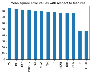
dtype: float64The bar plot below makes the winner obvious — RM (average rooms per dwelling) and LSTAT (lower-status population percentage) stand apart from the rest with much lower MSE values:
Build the reduced training and test sets using only the two best-performing features, RM and LSTAT:
X_train_2 = X_train[['RM', 'LSTAT']]
X_test_2 = X_test[['RM', 'LSTAT']]
Evaluating the Reduced Regression Model
Evaluate a LinearRegression trained on only the 2 selected features:
%%time
model = LinearRegression()
model.fit(X_train_2, y_train)
y_pred = model.predict(X_test_2)
print('r2_score: ', r2_score(y_test, y_pred))
print('rmse: ', np.sqrt(mean_squared_error(y_test, y_pred)))
print('sd of house price: ', np.std(y))r2_score: 0.5409084827186417
rmse: 6.114172522817782
sd of house price: 9.188011545278203
Wall time: 3 msNow train on all 13 original features as the baseline:
%%time
model = LinearRegression()
model.fit(X_train, y_train)
y_pred = model.predict(X_test)
print('r2_score: ', r2_score(y_test, y_pred))
print('rmse: ', np.sqrt(mean_squared_error(y_test, y_pred)))
print('sd of house price: ', np.std(y))r2_score: 0.5892223849182507
rmse: 5.783509315085135
sd of house price: 9.188011545278203
Wall time: 4 msWith just 2 features the model reaches an R² of 0.54 compared to 0.59 with all 13 — a reasonable result given that 11 features were discarded. The RMSE of 6.11 is well within one standard deviation of house prices (9.19), confirming that RM and LSTAT together capture the majority of the target signal.
Conclusion
In this tutorial you implemented univariate performance-based feature selection across two tasks. For the 370-feature classification dataset, you scored every feature by its individual ROC-AUC and reduced the set from 227 unique features to 11, cutting training time nearly in half while retaining 95.3% accuracy. For the Boston Housing regression dataset, you scored each of the 13 features by MSE from a single-feature linear regression and identified RM and LSTAT as the two most informative predictors.
Key takeaways:
- An ROC-AUC of exactly 0.5 means a feature performs no better than random guessing — any feature at or below that threshold can be dropped.
- MSE scores features by their individual linear fit to the target;
RMandLSTATachieved roughly half the error of every other Boston feature, making the selection clear-cut. - Removing constant, quasi-constant, and duplicate features first makes the per-feature scoring loop faster and avoids inflating the results with trivially useless columns.
- A small accuracy loss (0.58 pp in this case) is often acceptable in exchange for a significantly smaller feature set and faster training.
- This approach is model-agnostic for the scoring step — you can swap in any estimator to score features, as long as you apply the same estimator consistently across all features.
Next steps:
- Compare this metric-based approach with a statistical filter in Feature Selection Using Univariate ANOVA Test.
- Try information-theoretic scoring in Feature Selection Based on Mutual Information and Entropy Gain.
- Explore model-embedded selection in Lasso and Ridge Regularisation for Feature Selection.

